Motivation
Suppose you are trying to train a neural network to understand the following sentence:
"Ryan drove the car."
This sentence clearly has a different connotation from the following sentence:
"The car drove Ryan."
The human brain immideatly recognizes these difference. We can tell that in the first sentence a human drove the car, but in the second sentence there must be some artifical intelligence going on because the car is driving the human. Our brains have neurons with feedback connections, which can learn many behaviors and sequencing tasks. Thus, we can pick up on these differences very easily because we read each word in the sentence sequentially. We are picking up the context of each word from the words before it. Traditional neural networks would not differentiate the above two sentences, but a special type of network called a Long Short-Term Memory Network, a type of recurrent neural network, would be able to differentiate these two sentences. These types of networks are great for sequential taks like stock market prediction, music generation, speech recognition, and language detection.
Prerequisites
Before we talk about Long Short-Term Memory Networks, let us briefly cover a few prerequisites:
Feed Forward Neural Networks:
The goal of a feed forward neural network is to approximate some function $f^*$. For example, let $y = f^*(x)$ be a classifier which maps $x$ to a category $y$. The feed forward network defines a mapping $f(x;\theta) \rightarrow y$, which we can express as $f(x;\theta) = y$. This mapping learns the values of parameters of $\theta$, which result in the best approximation to the function $f^*$.
A feed forward network has inputs passing through hidden layers to generate outputs. Here, signals can only travel in the direction from input to output. The output layer does not affect the same or any other layer. We see an example as follows:
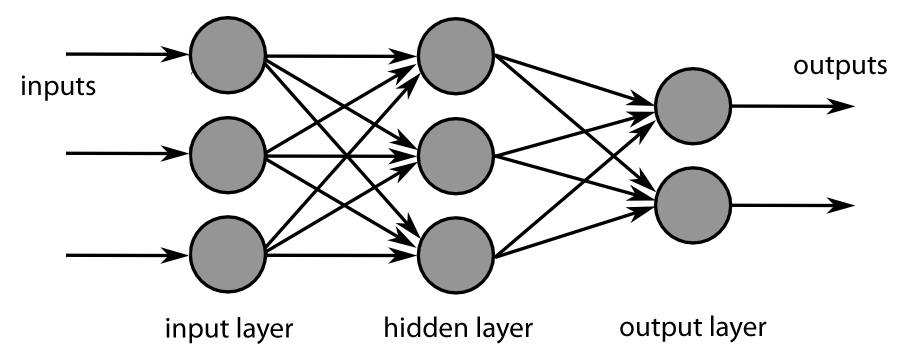
Above, we see that the input passes through the hidden layer which is then connected to the output layer to generate the outputs. The information is fed straight through, from left to right, never touching a given node twice.
Recurrent Neural Networks:
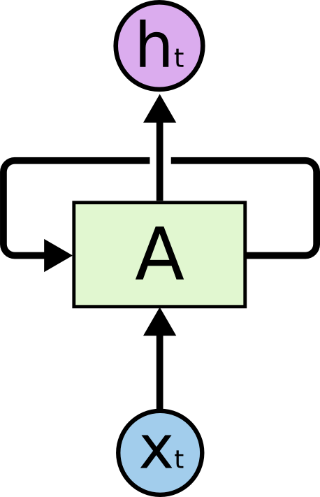
Recurrent neural networks (RNNs) are a family of neural networks for processing sequential data, a sequence of values $x^{(1)},x^{(2)},...,x^{(t)}$. In a traditional neural network, like the feed forward network above, we assume that all inputs and outputs are independent of each other. This is not the case for all tasks. If we are building a chat bot and want to predict the next word in reply, we need to know the words that came before it. Essentially, RNNs have memory. Every element in the sequence has the same task performed on it, with the output being dependant on the previous computations. An RNN looks as follows:
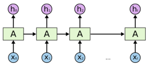
Here, we see that the sample $x_t$ is generated based on $x_0, x_1, ..., x_{t-1}$ and the output, $h_t$, is dependent on what comes before it. We see that the network forms loops. The first input is passed into its hidden layer and generates some output $h_0$. The second sequential input is passed into its hidden layer and so is the output from $h_0$. The activation function in hidden layer $h_1$ is activated on the second sample and this is then added with $h_0$. This process is then repeated until the last item in the sequence $x_t$. Traditionally, we depict this nature in the following image:
In the 1990's the vanishing gradient problem emerged as a major obstacle to RNN performance. The gradient expresses the change in all weights with respect to the change in error. Thus, not knowing the gradient foes not allow us to adjust the weigths in a direction taht will reduce the error. If we can't do this then the network will not learn. If any quantity is multiplied by a slightly larger quantity in a repeated fashion, the quantity can become very large. This is also true for the reverse case. If we multiply a quantity repeatedly by a quantity less than one, the quantity will become infitesimal. If this is hard to see, imagine that you are a gambler. You keep betting 1 dollar, but win 97 cents on that dollar every bet. You will soon see that this is not sustainable and you will go bankrupt very soon. The layers and timesteps in an RNN relate to each other through multiplication so the derivatives are susceptible to explosion or vanishing. For instance, let us look at multiple applications of the sigmoid in a repeated fashion:
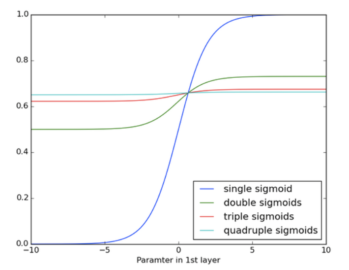
The sigmoid activation function is a popular activation in RNN's. We see here that the slope of the data becomes negligble and hence undetectable, thus vanishing.
RNN's were a great achievement. They were able to learn on sequential data where feed forward networks failed, but do suffer from the vanishing gradient problem.
History of the LSTM
In 1991, Dr. Jürgen Schmiduber and his former PhD student Sepp Hochreiter proposed a feedback network to overcome the vanishing and exploding gradient problem found with RNNs. In 1997, Schmidhuber and Hochreiter published the paper Long Short-Term Memory. In this paper they reivew Hochreiter's 1991 analysis of the problem of insufficient decaying error back flow in recurrent backpropogation. They combatted this problem by introducing the Long Short-Term Memory (LSTM). In the 90's, computing was still expensive and computing resources were not advanced, so LSTMs were not widely adopted. Fast forward 10 years and services like Amazon AWS and Microsoft Azure offered inexpensive computing which brought massive attention to LSTMs.
What are LSTMs?
Long Short-Term Memory networks are a type of recurrent neural network, which overcome the vanishing gradient problem found in a regular RNN. They typical LSTM has 3 main gates and a cell unit:
- Input Gate: The input gate controls how much of the newly computed state for the current input that you want to let through.
- Forget Gate: The forget gate defines how much of the previous state you want to let through.
- Output Gate: The output gate defines how much of the interant state you want to expose to the external network.
Mathematically, we can define these gates as equations as follows:
$$i_t = g(W_{x_i}x_t + W_{h_i}h_{t-1}+b_i)$$ $$f_t = g(W_{x_f}x_t + W_{h_f}h_{t-1}+b_f)$$ $$o_t = g(W_{x_o}x_t+W_{h_o}h_{t-1}+b_o)$$Above, $i_t$ is the input gate, $f_t$ is the forget gate, $o_t$ is the output gate, $g$ is a sigmoid activation function, $W$ represents a particular weight, and $b$ is a bias.
The cell unit can be transformed as:
$$ c_{in_t} = \text{tanh}\left(W_{xc}x_t + W_{hc}h_{t-1}+b_{c_{in}}\right)$$where $h_t = o_t \cdot \text{tanh} \left(c_t\right)$. The state can then be updated as:
$$c_t = f_t \cdot c_{t-1} + i_t \cdot c_{in_t}$$We can depict all of these equations graphically as:
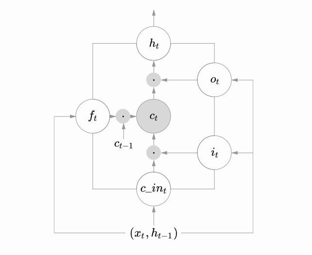
The gating allows the cell to keep pieces of information for prolonged periods of time while protecting the gradient inside the cell during training. This ensures that the gradient does not explode or vanish from multiple activations being processed.
Applications:
- Image Captioning - Oriol Vinyas, Alexander Toshev, Samy Bengio, and Dumitru Erhan published Show and Tell: A Neural Image Caption Generator. This paper uses an LSTM to automatically describe the content of an image.
- Hand Writing Generation - In 2014, Alex Graves published Generating Sequences With Recurrent Neural Networks. In this paper an LSTM model was used to generate handwriting from text. The handwriting was shown to be realistic cursive in a wide variety of styles.
- Stock Market Prediction - Tal Perry published the article Deep Learning the Stock Market. Here he used an LSTM to predict market prices.
- Movie Reviews - Jason Brownley published Sequence Classification with LSTM Recurrent Neural Networks in Python with Keras where he uses an LSTM to classify IMDB movie sentiment.
- Image Generation - In 2015, the Google DeepMind team published DRAW: A Recurrent Neural Network For Image Generation. This paper introduces the Deep Recurrent Attentive Writer, DRAW, which generates MNIST digits. DRAW was build with an LSTM layer.
- Reddit Comment Generator - Braulio Chavez published Reddit Comment Generator where he used LSTM cells to generate comments on Reddit.
Improving Performance of LSTMs:
To improve the performance of LSTMs we can attempt to do some of the following:
- Adding Regularization - Use l1, l2, or dropout layers.
- Bias - Adding a bias of 1 in every neuron in an LSTM layer has been noted to improve performance, drastically in some cases.
- Activation - Use softsign activation function over tanh. Also try softsign over softmax.
- Optimizers - RMSProp and AdaGrad are good choices for optimizers.
- Learning Rate - This parameter is very important, a well tuned learning rate can drastically improve performance.
- Data - Normalizing data can help. Also more data is always better because it helps combat overfitting.
Building our own LSTM:
Now that we have some background on LSTMs, let us build an LSTM for language detection. Hit the button below to jump to the next tutorial where we construct this LSTM using python, tensorflow, and keras.
References
- Images:
- Image 1 - http://coderoncode.com/machine-learning/2017/03/26/neural-networks-without-a-phd-part2.html
- Image 2 - http://colah.github.io/posts/2015-08-Understanding-LSTMs/
- Image 3 - http://colah.github.io/posts/2015-08-Understanding-LSTMs/
- Image 4 - https://deeplearning4j.org/lstm.html
- Image 5 - https://apaszke.github.io/lstm-explained.html
- Content:
- http://www.deeplearningbook.org/contents/rnn.html
- http://www.wildml.com/2015/10/recurrent-neural-network-tutorial-part-4-implementing-a-grulstm-rnn-with-python-and-theano/
- https://deeplearning4j.org/lstm.html
- http://colah.github.io/posts/2015-08-Understanding-LSTMs/
- https://en.wikipedia.org/wiki/Long_short-term_memory
- https://www.quora.com/What-are-the-various-applications-where-LSTM-networks-have-been-successfully-used