Introduction
If you are a frequent user of Google, you have probably seen this box before:
This is google translate. When you start typing in a sentence to translate, it automatically picks up the current language you are typing in. Let's test it out:
We see that we have typed in "bonjour", which means hello in french, and that google has automatically detected that our word is french. Here, Google uses recurrent neural networks to detect the current langauge and then translate it into the user's language of choice.
Language detection can be accomplished through Long Short-Term Memory. Let us take on the task of langauge detection using two datasets: a dataset consiting of english sentences and a dataset consitsting of french sentences.
Environment Setup
Below we have a description of each library we will use. Please click the links under installation and documentation to install and learn more about each library.
- Programming Language:
- Python 3 - Python is a general-purpose interpreted, interactive, object-oriented, and high-level programming language. We will be using version 3.x. This can be obtained from the official Python website or through the Anaconda distribution, which contains python 3 and many useful scientific computing libraries.
- Python Installation: Python Installation or Anaconda Installation
- Pip Installation: Pip Installation
- Libraries:
- TensorFlow - TensorFlow is an open-source software for machine intelligence. It is currently a very popular choice for developing deep learning modles.
- Installation: TensorFlow Installation
- Documentation: TensorFlow Documentation
- Numpy - Numpy is a package for scientific computing that contains many useful operations for a multi-dimensional data structure called an ndarray (np array).
- Installation: Numpy Installation
- Documentation: Numpy Documentation
- Matplotlib - Matplotlib, from the creators of numpy, is a plotting library that allows for custom charts like scatter plots, bar charts, line graphs, etc.
- Installation: Matplotlib Installation
- Documentation: Matplotlib Documentation
- Seaborn - Seaborn is an alternate plotting library that allows for easy construction of plots such as heatmaps.
- Installation: Matplotlib Installation
- Documentation: Matplotlib Documentation
- Scipy - Scipy, from the creators of numpy, is an alternate library for mathematics, science, and engineering.
- Installation: Scipy Installation
- Documentation: Scipy Documentation
- Sklearn - Sklearn has efficient tools for data mining, analysis, and machine learning.
- Installation: Sklearn Installation
- Documentation: Sklearn Documentation
- Random - Random allows us to create pseudo-random number generators for various distributions.
- Installation: Installed with Python
- Documentation: Random Documentation
Data
We will be detecting language between English and French. For this task, we will use the datasets found here. At this link there will be eng.txt and frn.txt. Both datasets contain sentences, in their respective language, from the Universal Declaration of Human Rights.
Imports
We start by importing the following libraries:
from __future__ import print_function;
import sys;
import random;
from random import randint

import numpy as np;

from keras.models import Sequential;
from keras.layers import Dense, Activation;
from keras.layers import LSTM;
from keras.optimizers import RMSprop;
from keras.utils.data_utils import get_file;
from keras.models import load_model;

from sklearn.cross_validation import train_test_split;
from sklearn.metrics import *;
from sklearn.externals import joblib;

import matplotlib.pyplot as plt;
from IPython.display import clear_output
from keras.callbacks import ModelCheckpoint, Callback

import subprocess;
import h5py;
Loading Data
Now that we have our English and French data, we need to load it. To do so we can open the filepath of the data and then use .read() to read it in. Additionally, we lower case the alphabet in the respective datafiles. Additionally, we will print the length of our English and French corpus so that we can see how much data we are dealing with. We do so as follows:
english_text = open('data/eng.txt').read().lower()
french_text = open('data/frn.txt').read().lower()

print('English corpus length:', len(english_text))
print('French corpus length:', len(french_text))

>>>
English corpus length: 10746
French corpus length: 12009
We see that our Engligh corpus has length 10746 and our French corpus has length 12009.
Character Set and Dictionary
Now that we have our English and French text loaded in we will need to obtain the character map for both datasets. To do so we can first create a set of the characters and then iterate over each character to create a dictionary where the keys are the characters and the values are integers from 0 to len(characters). Additionally, we create an inverse dictionary where the keys and values are flipped. The purpose of creating these dictionaries are to map the features to the feature indices in our upcoming design matrix. We do so as follows:
english_chars = sorted(list(set(english_text)))
french_chars = sorted(list(set(french_text)))

english_char_map = dict((c, i) for i, c in enumerate(english_chars))
french_char_map = dict((c, i) for i, c in enumerate(french_chars))

english_char_map_inverse = dict((i, c) for i, c in enumerate(english_chars))
french_char_map_inverse = dict((i, c) for i, c in enumerate(french_chars))
Sentence Creation
We now create sentences from both the English and French text, with a rolling window of 40 characters. These will serve as our features. To do so we set a maxlength of 40 and a step size of 3. We create an empty list for the sentences and an empty list for the next charaters. We then iterate over the length of the text minus the maxlength with a step size of 3 and append the text of the current character to 40 characters from that character. We also append the next character (character i + 40) to the next characters list. After doing so we will obtain an [x,40] matrix where each row will have length alphabet-size. We will additionally print the number of English and French sentences that we construct. We do so as follows:
maxlen = 40
step = 3

english_sentences = []
english_next_chars = []
for i in range(0, len(english_text) - maxlen, step):
    english_sentences.append(english_text[i: i + maxlen])
    english_next_chars.append(english_text[i + maxlen])

french_sentences = []
french_next_chars = []
for i in range(0, len(french_text) - maxlen, step):
    french_sentences.append(french_text[i: i + maxlen])
    french_next_chars.append(french_text[i + maxlen])

print('nb English sequences:', len(english_sentences))
print('nb French sequences:', len(french_sentences))

>>>
nb English sequences: 3569
nb French sequences: 3990
We see that we have created 3569 English sentences and 3990 French sentences.
Design Matrix Creation:
We can now vectorize the matrices we created above. Here, we create a feature matrix x, which is full of zeros and has size len(sentences),maxlength, character length. We will then let this matrix be of dtype boolean. We create a labels matrix y, full of zeros with size len(sentences), character length. This matrix is also of dtype boolean. We then iterate over the sentences and look at the t, char in the sentence. We set x[i,t,char_map[char]] = 1 in the inner loop and set y[i,char_map[next_chars[i]]] = 1. This will give us our vectorized features. We do so as follows:
char_len = max(len(english_chars), len(french_chars));

english_x = np.zeros((len(english_sentences), maxlen, char_len), dtype=np.bool)
english_y = np.zeros((len(english_sentences), char_len), dtype=np.bool)
for i, sentence in enumerate(english_sentences):
    for t, char in enumerate(sentence):
        english_x[i, t, english_char_map[char]] = 1
    english_y[i, english_char_map[english_next_chars[i]]] = 1


french_x = np.zeros((len(french_sentences), maxlen, char_len), dtype=np.bool)
french_y = np.zeros((len(french_sentences), char_len), dtype=np.bool)
for i, sentence in enumerate(french_sentences):
    for t, char in enumerate(sentence):
        french_x[i, t, french_char_map[char]] = 1
    french_y[i, french_char_map[french_next_chars[i]]] = 1
Train/Test Split:
Now that we have our Englisn and French features with their corresponding labels, we can use sklearn's train_test_split function to obtain a split of 80% training data and 20% testing data. Here, we will set a random_state = 1024. We do so as follows:
english_train_x, english_test_x, english_train_y, english_test_y = train_test_split(english_x, english_y, test_size=0.2, random_state=1024);
french_train_x, french_test_x, french_train_y, french_test_y = train_test_split(french_x, french_y, test_size=0.2, random_state=1024);
Now that we have our training and testing data, let us look at the shapes of the matrices.
print('English Shapes');
print(english_train_x.shape);
print(english_train_y.shape);
print(english_test_x.shape);
print(english_test_y.shape);
print()
print('French Shapes');
print(french_train_x.shape);
print(french_train_y.shape);
print(french_test_x.shape);
print(french_test_y.shape);

>>>
English Shapes
(2855, 40, 43)
(2855, 43)
(714, 40, 43)
(714, 43)

French Shapes
(3192, 40, 43)
(3192, 43)
(798, 40, 43)
(798, 43)
Above, we see that both languages have [x, 40, 43] values for training, even though French has 41 total alphabet charachters. We see this because we pad the smaller language with 2 extra columns of all 0s, in order to make sure that our neural network can train properly on the same input shape.
Generating Test Data:
The test split above was our holdout data. For the English and French holdout sets we will generate a new set of test data by randomly selecting 100 5-character substrings from each respective dataset. Here, we will end up with 200 strings, which will be our test features for evaluation. Our labels for the corresponding test data will have a 1 for English and a 0 for French. We will have 100 1's in the test labels and 100 0's. To create this test data we will create a function called random_generate(), which takes in our test data and a key. We start by creating two empty lists called labels, which will hold our labels, and feats, which will hold our features. We have a conditional that check if the key is "english" or "french". If the key is english then the labels vector will contain 100 1's. If it is french than the labels vector will contain 100 0's. We now iterate over range(100) and generate a random number between 0 and the length of the test data passed in. This will represent a random index to pull from inside the test data. We then generate another random integer between 0 and the length of the data in the index minus 5. This will represent a starting character. We can then extract this character plus the next 4 characters to obtain our random 5 character substring. We append this into the features variable. We will call this process for the English data and the French data and then combine the lists of the features and the lists of the labels and make each one a numpy array. We do so as follows:
def random_generate(test_x, key):
    labels = []
    feats = []
    if key == "english":
        labels = [1 for i in range(100)]
    elif key == 'french':
        labels = [0 for i in range(100)]
    else:
        return feats, labels;

    for i in range(100):
        r1 = randint(0, len(test_x) - 1)
        ind = test_x[r1]

        r2 = randint(0, len(ind) - 5)

        sub_string = ind[r2:r2+5]

        feats.append(sub_string)

    return feats,labels

english_sample, english_labels = random_generate(english_test_x, 'english')
french_sample, french_labels = random_generate(french_test_x, 'french')

test_data = np.array(english_sample + french_sample)
test_labels = np.array(english_labels + french_labels)
LSTM Model Creation:
Now that we have our training and test data, we can create our Long Short-Term Memory Model. To do so we will construct a function called build_model. This will set up a Sequential model with an LSTM layer that has 256 neurons followed by a dense layer that has shape number of characters (43) and a softmax activation function. Here we will use an RMSprop optimizer, with a leanring rate of 0.01, and a loss function of categorical_crossentropy. We create our function as follows:
def build_model(chars):
    print('Build model...')
    model = Sequential()
    model.add(LSTM(256, input_shape=(None, char_len)))
    model.add(Dense(char_len))
    model.add(Activation('softmax'))

    optimizer = RMSprop(lr=0.01)
    model.compile(loss='categorical_crossentropy', optimizer=optimizer, metrics=['accuracy'])
    return model
Prediction & Log Likelihood:
For each test string, we need to compute the log likelihood of that string for each model. To do so we will create a function called predict_on_sample which takes in a model and a test value. Here, we will iterate over each charachter, obtain the vector associated with it along with the previous START charachters, and obtain the prediction score for it on the next charachter. Finally, we sum up the logs of these values and return it. We create this function as follows:
def predict_on_sample(model, test_val):
    start = np.zeros((1, 1, char_len), dtype=bool)
    start_prob = model.predict(start)

    next_vec = start.copy()[0][0]
    probs = []

    probs.append(start_prob[0,np.argwhere(test_val[0])[0][0]])

    for idx, vec in enumerate(test_val):
        next_vec = np.append(next_vec, vec).reshape(1, idx+2, char_len)
        next_prob = model.predict(next_vec)

        probs.append(next_prob[0, np.argwhere(test_val[idx])[0][0]])

    return np.sum(np.log(probs))
ROC
Using the above function, we can predict the results on each test string. We can then create a function called predict_results(). We pass in the string along with both the English model and the French model, obtain the predicted probabilities, and compute the Generalized Likelihood Ratio Test (GLRT). The ratio gives us a vector of probability scores, in which we set all values >= 1 to 1, and otherwise 0. We can then obtain the false positive rate and true positive rate from the roc_curve function in the sklearn library and then use those to get the roc_auc from the auc function in sklearn. We create the function as follows:
def predict_results(english_model, french_model):
    english_preds = np.array([predict_on_sample(english_model, x) for x in test_data])
    french_preds = np.array([predict_on_sample(french_model, x) for x in test_data])
    ratio_probs = english_preds - french_preds

    fpr, tpr, _ = roc_curve(test_labels, ratio_probs);
    roc_auc = auc(fpr, tpr)

    print(roc_auc)

    return roc_auc, fpr, tpr
Now that we have the ROC, we can create a function called plot_roc_auc_curve to plot our ROC curve, which takes in the false positive rate, the true positive rate, the roc_auc, and a title. We create this function as follows:
def plot_roc_auc_curve(fpr, tpr, roc_auc, title):
    plt.figure()
    lw = 2
    plt.plot(fpr, tpr, color='darkorange',
             lw=lw, label='ROC curve (area = %0.2f)' % roc_auc)
    plt.plot([0, 1], [0, 1], color='navy', lw=lw, linestyle='--')
    plt.xlim([0.0, 1.0])
    plt.ylim([0.0, 1.05])
    plt.xlabel('False Positive Rate')
    plt.ylabel('True Positive Rate')
    plt.title('Receiver operating characteristic for ' + title)
    plt.legend(loc="lower right")
    plt.show()
Hyperparameter Tuning:
Above we have set up a functions to create our model LSTM model, obtain the predictions, compute the log likelihood, and compute the ROC. We have not instantiated the model yet as we do not know the optimal hyperparameters. Let us now perform a hyperparameter search. Previously, we wrote a function called train_and_predict(). We cycle though a set range of epochs and evaluate the model quality as the iterations increase. We then take the best performing model. Other hyperparameters tuned are the learning rate, decay rate, batch sizes used in training, and size of the LSTM layer. Some of these we tuned manually rather than create a automated function for it. Finally, we found that the best performance is given by epochs=8, learning rate=0.01, decay=0.0, layer_size=256.
Below we display graphs showing the loss vs. epochs and accuracy vs. epochs for learning rate 0.01 as a demonstration of our parameter selection process.


Building English & French LSTM Models
Let us create our English and French LSTM models with 5 epochs, a step size of 5, and an optimal batch size of 2512:
models_1 = train_and_predict(5, 5, 2512)

>>>
Build model...
Build model...
Epoch 1/5
2855/2855 [==============================] - 3s - loss: 3.7206 - acc: 0.0221
Epoch 2/5
2855/2855 [==============================] - 2s - loss: 5.3884 - acc: 0.1426
Epoch 3/5
2855/2855 [==============================] - 2s - loss: 4.2558 - acc: 0.0676
Epoch 4/5
2855/2855 [==============================] - 2s - loss: 3.5550 - acc: 0.1625
Epoch 5/5
2855/2855 [==============================] - 2s - loss: 3.4811 - acc: 0.0550
Epoch 1/5
3192/3192 [==============================] - 3s - loss: 3.8357 - acc: 0.0711
Epoch 2/5
3192/3192 [==============================] - 2s - loss: 3.4972 - acc: 0.0655
Epoch 3/5
3192/3192 [==============================] - 2s - loss: 4.1910 - acc: 0.1103
Epoch 4/5
3192/3192 [==============================] - 2s - loss: 3.0199 - acc: 0.0840
Epoch 5/5
3192/3192 [==============================] - 2s - loss: 2.9137 - acc: 0.1732
0.7948
We see that this configuration has given us an ROC of 0.7948.
Let us now create our LSTM models with 12 epochs, a step size of 3 epochs, and a batch size of 2512:
models_2 = train_and_predict(12, 3, 2512)

>>>
Build model...
Build model...
Epoch 1/3
2855/2855 [==============================] - 3s - loss: 3.8244 - acc: 0.0319
Epoch 2/3
2855/2855 [==============================] - 2s - loss: 3.8091 - acc: 0.0501
Epoch 3/3
2855/2855 [==============================] - 2s - loss: 4.0902 - acc: 0.0630
Epoch 1/3
3192/3192 [==============================] - 4s - loss: 3.6929 - acc: 0.0592
Epoch 2/3
3192/3192 [==============================] - 2s - loss: 4.6424 - acc: 0.1419
Epoch 3/3
3192/3192 [==============================] - 2s - loss: 4.5772 - acc: 0.0617
0.8456
Epoch 1/3
2855/2855 [==============================] - 2s - loss: 3.1018 - acc: 0.1625
Epoch 2/3
2855/2855 [==============================] - 2s - loss: 3.0159 - acc: 0.1541
Epoch 3/3
2855/2855 [==============================] - 2s - loss: 3.0308 - acc: 0.1625
Epoch 1/3
3192/3192 [==============================] - 2s - loss: 3.7905 - acc: 0.1604
Epoch 2/3
3192/3192 [==============================] - 2s - loss: 3.7677 - acc: 0.1554
Epoch 3/3
3192/3192 [==============================] - 2s - loss: 3.7589 - acc: 0.1560
0.8479
Epoch 1/3
2855/2855 [==============================] - 2s - loss: 3.0133 - acc: 0.1625
Epoch 2/3
2855/2855 [==============================] - 2s - loss: 2.9974 - acc: 0.1604
Epoch 3/3
2855/2855 [==============================] - 2s - loss: 2.9674 - acc: 0.1625
Epoch 1/3
3192/3192 [==============================] - 2s - loss: 3.6747 - acc: 0.1538
Epoch 2/3
3192/3192 [==============================] - 2s - loss: 3.7156 - acc: 0.1441
Epoch 3/3
3192/3192 [==============================] - 2s - loss: 3.7864 - acc: 0.1444
0.865
Epoch 1/3
2855/2855 [==============================] - 2s - loss: 2.9449 - acc: 0.1653
Epoch 2/3
2855/2855 [==============================] - 2s - loss: 2.9600 - acc: 0.1520
Epoch 3/3
2855/2855 [==============================] - 2s - loss: 3.0080 - acc: 0.1891
Epoch 1/3
3192/3192 [==============================] - 2s - loss: 3.7089 - acc: 0.1598
Epoch 2/3
3192/3192 [==============================] - 2s - loss: 3.6826 - acc: 0.1526
Epoch 3/3
3192/3192 [==============================] - 2s - loss: 3.7564 - acc: 0.1507
0.8629
Here, we see that our ROC is now 0.8629, which is much better than that of the model that used 5 epochs.
We note that there is a lof of variability in model performance. We noticed that our ROC varied from 0.65 to 0.95. Thus, we have re run our above model generation code multiple times and have saved the best performing model. Below we save these best performing models:
models_1[3][0].save('model_current_e.h5')
models_1[3][1].save('model_current_f.h5')
We can now load the best performing models:
model_1 = load_model('model_current_e.h5')
model_2 = load_model('model_current_f.h5')
Model Performance:
We can now call our functions to obtain the ROC, false positive rate, true positive rate. We call our function with our models as follows:
roc, fpr, tpr = predict_results(model_1, model_2)

>>>
0.9476
Here we see that we have achieved a great ROC of 0.9476.
Let us now plot our ROC curve:
plot_roc_auc_curve(fpr, tpr, roc, 'English/French Classification')

>>>
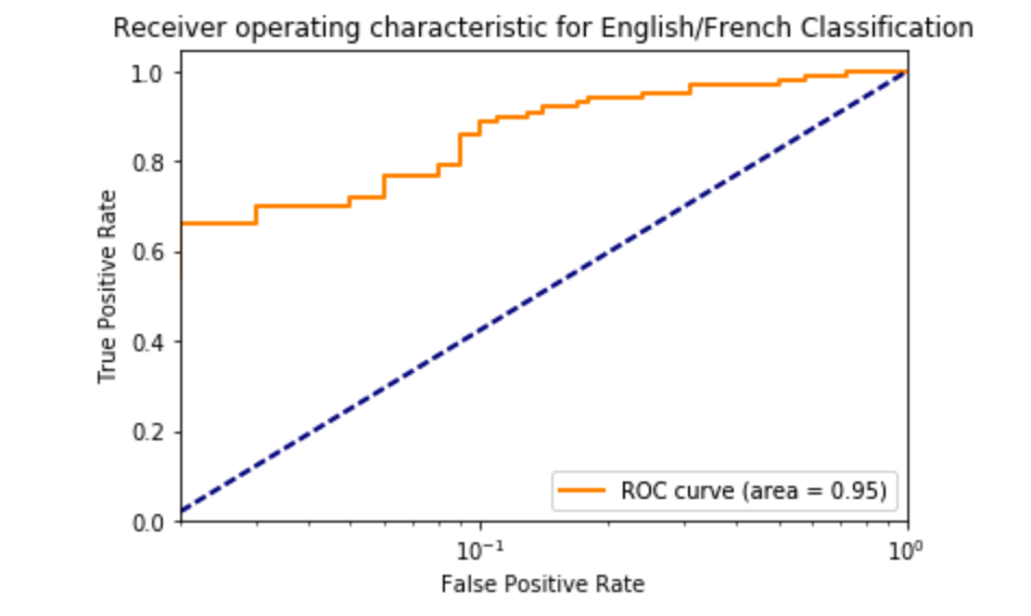
We see that the above ROC curve looks great.
Questions
- Is this model good? We believe that our model is good. Our model was able to produce an ROC of 0.9476, where a 1.0 is the highest possible ROC score. To achieve this ROC, we tuned our parameters and trained our Neural Network on the best set of parameters we found. The measure of accuracy is also dependent on the test examples we use for evaluation. While training and testing our model, we saw that there were some examples which were more difficult to distinguish between languages than others. Using a sample from those test examples yielded worse ROC, around 0.65, but some examples gave us above 0.95 ROC. Despite the variability in these results, the lower limit of our ROC is still very high, which shows that our model performs well.
- What are 3 Alternatives to language detection with their pros and cons?
- Naive Bayes Classification - Textblob is a popular python module for processing text data using natural language processing. In particular, they have a language detector that is built using a Naive Bayes Classifier, which can pass in a feature extractor as a parameter. Information on how to build this langauge detector can be found here. In this example, a feature extractor that uses the last letter of a given word is used. This seems very simple, but achieved an accuracy of 0.7 on the test set. They had found that words that do not end with the letter “o” tend to be English. The pros of this approach is that the naive bayes classifier works very well with high dimensions and is computationally inexpensive. This would allow us to create a custom feature extractor that has very high dimensionality but still runs in a reasonable amount of time. The cons of their approach is that the feature here is weak. Using only the last letter of each word does not seem to build a great feature. There are many words that end with the same letter in across multiple languages so this might not work well for languages that are fairly similar. Additionally, a con with regards to a naive bayes classifier is that it relies on an independence assumption. If this assumption is not met the classifier will perform badly.
- N-Grams - Mark Galea implemented Language Detection using N-Grams in this post. An N-gram is an N-character slice of a longer string. He notes that words that appear in the English language are clearly different than words that appear in the French language and that the set of N-grams will be different for each language. Further he notes that if a language detector is used on small fragments of text then there is less susceptibility to noise which makes the language detector more resilient. Galea uses the following preprocessing steps in his N-Gram language detector:
- Remove extra spaces
- Discard digits and punctuation except apostrophes
- Tokenize
- Generate train/test split
- Scan down each token generating all possible N-grams for N = 1 - 5
- Create a hash table
- Logistic Regression - Language detection using Logistic Regression has also been implemented by Bugro here. This approach takes advantage of language roots, such as prefixes and suffixes, and creates features based on them. These features are then used to train a Logistic Regression model that gives high accuracy on the problem of classification. There are a few advantages of this. One is that it takes advantage of parts of a word that contribute more to a model than those that don't. For instance, verbs in the english language usually end in 'ing', 'ed', and other tenses, but french verbs have 'ais' and 'ent'. By training on specifically these types of features, we can increase the accuracy of the model. However, this advantage is offset by using a Logistic model as the primary classifier. It is difficult to justify the linearity of this problem, and logistic regression relies on the linear separability of a problem. To overcome this significant disadvantage, we can use kernels and regularization. Kernels can be applied to a logistic regression classifier to fit a non-linear classifiable dataset. Regularization, on the other hand, can be used to reduce the variance of our classifier, at the cost of introducing more bias. This is actually one of the main problems with our Neural Network model. It's high variance is evident in the results that range from 65% to 95% ROC, which a Logistic Regression model trained on word roots should be able to overcome.
- What are 5 ways in which we could improve our model?
- More Data - Having more training and testing data is always better, espeically when we are using deep learning. We had 3569 total English sentences to work with and 3990 French sentences to work with. This is not a huge dataset. Having more data from each dataset would allow us to better train our model to better represent the actual population of the data. If we had more text that looked like English or French our model would be able to better understand the English features compared to the French features. However, more data would increase the computational expense for our model. This task already had some expense to it and adding multiple times the amount of data would drastically increase the runtime. We believe that having more data would drop our ROC slightly as we would better be able to represent the English and French populations, but our computational expense would be mich higher.
- Alternate Layers - Our model had an LSTM layer and a dense layer. Here, we did not explore the possibility of adding alternate layers such as a dropout layer. A droput layer is a powerful regularization technique. Here, neurons that are randomly selected are ignored during training. This allows our network to be less sensitive to the specific weights of neurons. Thus, our network is capable of better generalization and is less likely to overfit the training data. Less overfitting is definitely a pro. Adding and experimenting with different layers can help improve performance, but a con is that this would add computational expense to our program in terms of runtime and in human labor as we would have to find the optimal hyperparameters for the layers. Also, this is not guranteed to help in terms of performance. It may very well be that our network performs worse with a dropout layer or a different layer structure. We believe that adding a dropout layer would prevent overfitting and that experimenting with layers could boost performance in terms of accuracy, precision, recall, and AUC.
- Different Optimizer - In our model we used an RMSprop optimizer with a learning rate of 0.01. We did not try alternate optimization techniques such as SGD, Adagrad, Adadelta, Adam , etc. With regards to Long Short-Term Memory, Adam and Adadelta usually are a fine choice. We tuned the learning rate for the RMSprop, but did not experiment with these alternate optimizers. Potentially, we could have achieved better performance or converged more quickly than with our choice of optimizer. However, it is not guranteed that a different optimizer would drastically improve the performance. Also, it might take longer to converge than our choice of optimizer. Additionally, running experiments with these would take additional time. We do not think that the optimizer choice would make a huge difference in performance, but we do think that some optimizers are better suited for tasks than others. Thus, we think that we could converge faster using an optimizer such as Adam. This would allow us to run less epochs and decrease our computational expense.
- Bias - Adding a bias of 1 has been shown to help improve the performance and prevent overfitting especially in regards to LSTM models. When we created our LSTM in keras we did not set use_bias = True. Having this bias vector could have lead to less overfitting in our model. A con would be that our ROC could potentially drop and our model would not look as good as it does. We think that adding bias is a great idea, which would help prevent our model from overfitting, but would drop our ROC. In this case this is fine because we want user querys to be as accurate as possible. Using a bias could potentially achieve this.
- More Epochs - We used a maximum of 12 epochs when we trained our model. Using a GPU allows for more training in a smaller time frame. Instead of running 12 epochs we could have run 100. Running this experiment and obtaining shorter run time is definitely a positive, but a con would be that the model converges after a few iterations and there is no gained preformance by using the GPU to run more epochs. We think that we could run more epochs, but we would have no change in efficacy. We saw that there was convergence across 8-10 epochs as the derivative of the loss started became somwhat constant from iteration to iteration. However, GPUs allow for much faster training.
Extra Credit:
In extension to our previously developed language detection model for English vs French, we will now explore a 10-way langauge comparison of both traditional western langauges as well as non-Latin based langauges. The languages we are utilizing are as follows:
- English
- French
- Dutch
- German
- Italian
- Latin
- Portugese
- Japanese
- Russian
- Spanish
We will create LSTM models for each language and tune the set of optimal hyperparameters found in the English-French LSTM comparison in the previous notebook. There, we evaluated learning rate, decay, batch size, LSTM layer size, and number of epochs. In order to train our 10 models efficiently we spun up a Microsoft Azure NC12 which has 12 cores, 120 GiB ram, and 2 K80 GPUs. This will allow us to run over 2000 epochs in less than two hours. After doing so we will examine the ROC for pairs of language models and be able to determine which paris of langauges our model was able to distinguish best and which languages our models were not able to distingush.
Imports
We import the following libraries:
from __future__ import print_function;
import re;
import sys;
import random;
import unicodedata;
from random import randint;

import numpy as np;
import seaborn as sns;

from keras.models import Sequential;
from keras.layers import Dense, Activation;
from keras.layers import LSTM;
from keras.optimizers import RMSprop;
from keras.utils.data_utils import get_file;
from sklearn.cross_validation import train_test_split;
from sklearn.metrics import *;
from sklearn.externals import joblib;

import matplotlib.pyplot as plt;
from IPython.display import clear_output
from keras.callbacks import ModelCheckpoint, Callback

import subprocess;
import h5py;
Notifications:
Since we will be running many epochs across many different languages we have set up a slack channel to push notifications when functions finish running. This will help monitor the status of our program. We create a function called notify_slack which takes in a text to be sent to our channel. We create it as follows:
def notify_slack(text):
    text = 'WebSearch: ' + text;
    subprocess.Popen('''curl -X POST --data-urlencode "payload={'channel' : '#random', 'username': 'webhookbot', 'text':'''+ '\'' + text + '\'' + '''}" https://hooks.slack.com/services/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''', shell=True)
Data Cleaning:
Our data might originally be messy and contain accents that are not held within English alpha-numeric characters. Thus, we will create a function called strip_accents which takes in a string to remove these characters to avoid giving cerain models an unfair advantage. Inside this function we use the unicodedata.normalize function on our given strings with an appropriate code. We do so as follows:
def strip_accents(s):
    return ''.join(c for c in unicodedata.normalize('NFD', s)
                   if unicodedata.category(c) != 'Mn')
Loading Data:
In order to use languages with a non-Latin scrip, we first need to transliterate them into traditional Enlgish. We've used this link to Romanize Russian and this link to Romanize Japanese. Additionally, we stripped out these non-translated characters: 及, 受, 胞, 認. We can now load our language datasets. Here we first create a list of all our langauge txt files. Additionally, we create a list with their respective names. We'll keep languagaes in this order for all of our datasets for simplicity. We strip accents, lower case each character and add it to an overall list of languages.
languages = ['data/eng.txt',
             'data/frn.txt',
             'languages/dut.txt',
             'languages/ger.txt',
             'languages/itn.txt',
             'languages/ltn.txt',
             'languages/por.txt',
             'languages/romanized_jap.txt',
             'languages/romanized_rus.txt',
             'languages/spn.txt' ]

language_names = ['English',
                  'French',
                  'Dutch',
                  'German',
                  'Italian',
                  'Latin',
                  'Portugese',
                  'Japanese',
                  'Russian',
                  'Spanish']

all_text = []
for file in languages:
    text = open(file).read().lower()
    all_text.append(strip_accents(text))

for text in all_text:
    print(text[0:20])

>>>
universal declaratio
declaration universe
universele verklarin
resolution 217 a (ii
il 10 dicembre 1948,
declarationem homini
declaracao universal
'sekai jinken sengen
vseobsaja deklaracij
declaracion universa
Character Set & Dictionary
We now need to obtain a set of all of the characters in our language, a dictionary that maps each character to an integer, and a dictionary that maps integers to the characters. To do so we can iterate over all of our languages text in all_data and create a set of the characters in the text for each language. We can then append this into all_chars. In all_char_map we can create a dictionary with the keys as the elements in the sorted set and the values as integers from 0 to len(sorted_characters). We can then append this dictionary into the list all_char_map. We then swap the keys and values in the all_char_map dictionary and append this into all_char_map_inverse. We do so as follows:
all_chars = []
all_char_map = []
all_char_map_inverse = []
for idx, lang in enumerate(all_text):
    all_chars.append(sorted(list(set(lang))))
    all_char_map.append(dict((c, i) for i, c in enumerate(sorted(list(set(lang))))))
    all_char_map_inverse.append(dict((i, c) for i, c in enumerate(sorted(list(set(lang))))))

    print (language_names[idx])
    print ("\tCorpus length:", len(lang))
    print ("\tCharacter Count", len(all_chars[idx]))
    print ()

>>>
English
    Corpus length: 10746
    Character Count 43

French
    Corpus length: 12009
    Character Count 41

Dutch
    Corpus length: 12887
    Character Count 42

German
    Corpus length: 12078
    Character Count 45

Italian
    Corpus length: 12768
    Character Count 39

Latin
    Corpus length: 10065
    Character Count 32

Portugese
    Corpus length: 11459
    Character Count 42

Japanese
    Corpus length: 11551
    Character Count 38

Russian
    Corpus length: 12240
    Character Count 43

Spanish
    Corpus length: 12078
    Character Count 42
We can now create our sentences like we previously did for our English and French models:
maxlen = 40
step = 3

all_sentences = []
all_next_chars = []

for idx, lang in enumerate(all_text):
    sentences = []
    next_chars = []
    for i in range(0, len(lang) - maxlen, step):
        sentences.append(lang[i: i + maxlen])
        next_chars.append(lang[i + maxlen])

    all_sentences.append(sentences)
    all_next_chars.append(next_chars)

    print (language_names[idx])
    print ("\tSentences:", len(sentences))
    print ()

>>>
English
    Sentences: 3569

French
    Sentences: 3990

Dutch
    Sentences: 4283

German
    Sentences: 4013

Italian
    Sentences: 4243

Latin
    Sentences: 3342

Portugese
    Sentences: 3807

Japanese
    Sentences: 3837

Russian
    Sentences: 4067

Spanish
    Sentences: 4013
Design Matrix Creation
We will now vectorize the above matrices by creating a design matrix. This will result in an [x, 40, max-alphabet-length] shape matrix for each langauge. We do so like we did for the English and French models:
char_len = max([len(x) for x in all_chars])

all_x = []
all_y = []

for idx, lang in enumerate(all_text):
    x = np.zeros((len(all_sentences[idx]), maxlen, char_len), dtype=np.bool)
    y = np.zeros((len(all_sentences[idx]), char_len), dtype=np.bool)

    for i, sentence in enumerate(all_sentences[idx]):
        for t, char in enumerate(sentence):
            x[i, t, all_char_map[idx][char]] = 1
        y[i, all_char_map[idx][all_next_chars[idx][i]]] = 1

    all_x.append(x)
    all_y.append(y)
Train/Test Split:
We now use sklearn's train_test_split function to create an 80% training set and 20% testing set for our data.
all_train_x = []
all_test_x = []
all_train_y = []
all_test_y =[]

for idx, lang in enumerate(all_text):
    train_x, test_x, train_y, test_y = train_test_split(all_x[idx], all_y[idx], test_size=0.2, random_state=1024);
    all_train_x.append(train_x)
    all_test_x.append(test_x)
    all_train_y.append(train_y)
    all_test_y.append(test_y)
Generate Testing Data:
Having obtained the test split, we need to obtain a smaller sample of 100 strings of 5 length charachters each. We do this by using a Random number generator to select a random string each time, append it to our features array, along with the label associated with it. In orde to compare two languages, we had to make changes to the language generation method. We take two random seeds to create random generators. We seed them in such a way to ensure that the language in the first pair has the same text for each language it is compared to and similarly for the second pair. This also ensures that when we compare English to English, we use two different test samples. For example, the same English text will be compared to all other languages. Then when we compare all other languages to English we still use the same English text sample. This ensures the maximum variability in our language detection scheme.
def random_generate(test_x_1, test_x_2, seed_1, seed_2):
    both_labels = []
    both_feats = []

    rands = [random.Random(), random.Random()]

    rands[0].seed(seed_1)
    rands[1].seed(sys.maxsize - seed_2)


    key = 1
    for test_x in [test_x_1, test_x_2]:
        labels = []
        feats = []
        for i in range(100):
            r1 = rands[key].randint(0, len(test_x) - 1)

            ind = test_x[r1]
            r2 = rands[key].randint(0, len(ind) - 5)

            sub_string = ind[r2:r2+5]

            feats.append(sub_string)
            labels.append(key)

        both_labels.append(labels)
        both_feats.append(feats)
        key = key^1

    return both_feats, both_labels
With out above function we can now call it for all pairs of languages and append them into a samples and labels list:
all_samples_1 = []
all_labels_1 = []

all_samples_2 = []
all_labels_2 = []

for idx, test_x in enumerate(all_test_x):
    for idx2, test_x2 in enumerate(all_test_x):

        [[feats_1, feats_2], [labels_1, labels_2]] = random_generate(test_x, test_x2, idx, idx2)
        all_samples_1.append(feats_1)
        all_labels_1.append(labels_1)

        all_samples_2.append(feats_2)
        all_labels_2.append(labels_2)
LSTM Model Creation:
Now that we have obtained our data for training and testing, we will build a LSTM model. To do this, we will create a function that will build a Sequential LSTM model. The parameters for the model below have been tuned after testing multiple configurations with over 60 epochs each. We settled on using 256 Neurons on the LSTM layer, with a RMSProp optimizer using 0.01 Learning rate. We will show our results on how we obtained these values later.
def build_model(chars):
    print('Build model...')
    model = Sequential()
    model.add(LSTM(256, input_shape=(None, char_len)))
    model.add(Dense(char_len))
    model.add(Activation('softmax'))

    optimizer = RMSprop(lr=0.01)
    model.compile(loss='categorical_crossentropy', optimizer=optimizer, metrics=['accuracy']);
    return model
Prediction & Log Likelihood:
To do a prediction on our data, we will use a log of probabilities over each charachter in a string. We will iterate over each charachter, obtain the vector associated with it along with the previous START charachters, and obtain the prediction score for it on the next charachter. Finally, we sum up the logs of these values and return it.
def predict_on_sample(model, test_val):
    start = np.zeros((1, 1, char_len), dtype=bool);
    start_prob = model.predict(start);

    next_vec = start.copy()[0][0];
    probs = [];

    probs.append(start_prob[0,np.argwhere(test_val[0])[0][0]]);

    for idx, vec in enumerate(test_val):
        next_vec = np.append(next_vec, vec).reshape(1, idx+2, char_len)
        next_prob = model.predict(next_vec);

        probs.append(next_prob[0, np.argwhere(test_val[idx])[0][0]]);

    return np.sum(np.log(probs));
Using the above function, we can predict the results on each test string. To do this, we pass in the string along with both the English model and the French model, obtain the probabilities, and compute the GLRT. The ratio gives us a vector of probability scores, in which we set all values >= 1 to 1, and otherwise 0. The ROC score can then be computed on these values.
ROC
We can use the same function predict_results that we built in Part 1 to obtain the ROC score, false positive rate, and true positive rate. We do so as follows:
def predict_results(model_1, model_2, lang_idx_1, lang_idx_2):

    test_data = np.array(all_samples_1[lang_idx_1] + all_samples_2[lang_idx_2]);
    test_labels = np.array(all_labels_1[lang_idx_1] + all_labels_2[lang_idx_2]);

    preds_1 = np.array([predict_on_sample(model_1, x) for x in test_data]);
    preds_2 = np.array([predict_on_sample(model_2, x) for x in test_data]);

    ratio_probs = preds_1 - preds_2;

    fpr, tpr, _ = roc_curve(test_labels, ratio_probs);
    roc_auc = roc_auc_score(test_labels, ratio_probs);

    return roc_auc, fpr, tpr;
Hyperparameter Tuning:
We use the same hyperparameters as we did in the first section. Here we did an entense search wich gave us an ROC of ~0.95 for our English and French models. For more details on this please read the above hyperparameter tuning section.
Building Models:
We create a function called train_and_predict to build two models for each respective language, fit the training data, predict the results, and obtain the roc. The function is as follows:
def train_and_predict(lang_idx_1, lang_idx_2, total_epochs, batch_size=2048):
    model_1 = build_model(all_chars[lang_idx_1])
    model_2 = build_model(all_chars[lang_idx_2]);

    epochs_ran = 0;

    history_1 = model_1.fit(all_train_x[lang_idx_1], all_train_y[lang_idx_1],
                        batch_size=batch_size, epochs=total_epochs, shuffle=True, verbose=0);
    history_2 = model_2.fit(all_train_x[lang_idx_2], all_train_y[lang_idx_2],
                        batch_size=batch_size, epochs=total_epochs, shuffle=True, verbose=0);

    roc, _, _ = predict_results(model_1, model_2, lang_idx_1, lang_idx_2);


    return roc, history_1, history_2, model_1, model_2;
We can now run each of our 100 models for comparisons between every language. We then save them to a 5-tuple of outputs which we represent as a variable called all_models.
all_models = []
for idx, lang in enumerate(all_text):
    model_results = []
    for idx_2, lang2 in enumerate(all_text):
        result = train_and_predict(lang_idx_1=idx, lang_idx_2=idx_2, total_epochs=8, batch_size=2512)
        model_results.append(result)
        print ("Finished: %s -> %s with ROC=%f" % (language_names[idx], language_names[idx_2], result[0]))
    all_models.append(model_results)
    notify_slack("Finished all models for " + language_names[idx])
Model Evaluation:
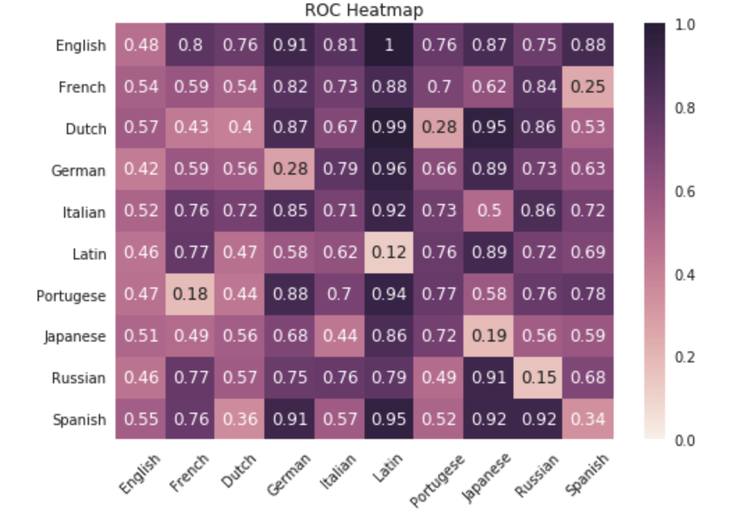
Next, we extract the loss and the ROC of each language combination. We've printed the ROCs below so they can be read easily and then create a heat map to give a graphical representation of how languages compare to each other.
all_roc = dict()
all_roc_list = []

all_fpr = dict()
all_tpr = dict()
all_loss = []

for idx_1 in range(len(all_models)):
    language_roc = []
    language_loss = []

    for idx_2 in range(len(all_models[idx_1])):
        roc, history_1, history_2, model_1, model_2 = all_models[idx_1][idx_2]
        roc_auc, fpr, tpr = predict_results(model_1, model_2, idx_1, idx_2)

        index = idx_1*len(all_models) + idx_2
        all_roc[index] = roc_auc
        all_fpr[index] = fpr
        all_tpr[index] = tpr

        language_roc.append(roc_auc)
        language_loss.append(history_2.history["loss"][-1])

        print ("%s - %s ROC: %f" % (language_names[idx_1], language_names[idx_2], roc_auc))
    print()

    all_roc_list.append(language_roc)
    all_loss.append(language_loss)

>>>
English - English ROC: 0.477350
English - French ROC: 0.802600
English - Dutch ROC: 0.755800
English - German ROC: 0.908600
English - Italian ROC: 0.810800
English - Latin ROC: 0.998000
English - Portugese ROC: 0.762200
English - Japanese ROC: 0.867500
English - Russian ROC: 0.749200
English - Spanish ROC: 0.882100

French - English ROC: 0.539400
French - French ROC: 0.591300
French - Dutch ROC: 0.540000
French - German ROC: 0.821700
French - Italian ROC: 0.730300
French - Latin ROC: 0.876100
French - Portugese ROC: 0.700300
French - Japanese ROC: 0.619500
French - Russian ROC: 0.839700
French - Spanish ROC: 0.249700

Dutch - English ROC: 0.569900
Dutch - French ROC: 0.427800
Dutch - Dutch ROC: 0.403100
Dutch - German ROC: 0.872900
Dutch - Italian ROC: 0.673000
Dutch - Latin ROC: 0.993700
Dutch - Portugese ROC: 0.280700
Dutch - Japanese ROC: 0.954800
Dutch - Russian ROC: 0.862400
Dutch - Spanish ROC: 0.532500

German - English ROC: 0.419550
German - French ROC: 0.589200
German - Dutch ROC: 0.562500
German - German ROC: 0.275900
German - Italian ROC: 0.791100
German - Latin ROC: 0.960000
German - Portugese ROC: 0.656000
German - Japanese ROC: 0.888800
German - Russian ROC: 0.731600
German - Spanish ROC: 0.634300

Italian - English ROC: 0.523200
Italian - French ROC: 0.764300
Italian - Dutch ROC: 0.718100
Italian - German ROC: 0.851100
Italian - Italian ROC: 0.710600
Italian - Latin ROC: 0.921500
Italian - Portugese ROC: 0.729000
Italian - Japanese ROC: 0.496600
Italian - Russian ROC: 0.859700
Italian - Spanish ROC: 0.719200

Latin - English ROC: 0.459950
Latin - French ROC: 0.774300
Latin - Dutch ROC: 0.474000
Latin - German ROC: 0.582900
Latin - Italian ROC: 0.620700
Latin - Latin ROC: 0.122300
Latin - Portugese ROC: 0.759200
Latin - Japanese ROC: 0.889800
Latin - Russian ROC: 0.722400
Latin - Spanish ROC: 0.687900

Portugese - English ROC: 0.465650
Portugese - French ROC: 0.181500
Portugese - Dutch ROC: 0.440800
Portugese - German ROC: 0.883500
Portugese - Italian ROC: 0.704400
Portugese - Latin ROC: 0.940300
Portugese - Portugese ROC: 0.765300
Portugese - Japanese ROC: 0.581000
Portugese - Russian ROC: 0.762200
Portugese - Spanish ROC: 0.781800

Japanese - English ROC: 0.509550
Japanese - French ROC: 0.491700
Japanese - Dutch ROC: 0.558000
Japanese - German ROC: 0.684700
Japanese - Italian ROC: 0.440500
Japanese - Latin ROC: 0.860400
Japanese - Portugese ROC: 0.719100
Japanese - Japanese ROC: 0.185900
Japanese - Russian ROC: 0.558600
Japanese - Spanish ROC: 0.587150

Russian - English ROC: 0.456500
Russian - French ROC: 0.767000
Russian - Dutch ROC: 0.567500
Russian - German ROC: 0.753800
Russian - Italian ROC: 0.762700
Russian - Latin ROC: 0.789500
Russian - Portugese ROC: 0.485850
Russian - Japanese ROC: 0.912000
Russian - Russian ROC: 0.153200
Russian - Spanish ROC: 0.682300

Spanish - English ROC: 0.553750
Spanish - French ROC: 0.764800
Spanish - Dutch ROC: 0.361900
Spanish - German ROC: 0.912800
Spanish - Italian ROC: 0.567100
Spanish - Latin ROC: 0.953900
Spanish - Portugese ROC: 0.519700
Spanish - Japanese ROC: 0.917700
Spanish - Russian ROC: 0.917300
Spanish - Spanish ROC: 0.342050
To see these easier we can create a heatmap to display the ROC's for each langauge. We do so as follows:
sns.set()
ax = sns.heatmap(all_roc_list, vmin=0, vmax=1, annot=True, yticklabels=language_names, xticklabels=language_names)
plt.xticks(rotation=45)
plt.title("ROC Heatmap")
sns.plt.show()

>>>
We can also generate an ROC curve to plot multiple ROC curves on the same graph. This will allow us to visualize all ROC's together:
def plot_roc_auc(fpr_, tpr_, roc_, title, num_plot):
    plt.figure(figsize=(10,12))

    language_pairs = []
    for lang in language_names:
        for lang2 in language_names:
            language_pairs.append(lang[0:3]+"-"+lang2[0:3])

    lw=1.15
    for i in range(num_plot):
        plt.plot(fpr_[i], tpr_[i], lw=lw,
                 label='{0} (area = {1:0.2f})'
                 ''.format(language_pairs[i], roc_[i]))

    plt.plot([0, 1], [0, 1], 'k--', lw=lw)
    plt.xlim([0.0, 1.0])
    plt.ylim([0.0, 1.05])
    plt.xlabel('False Positive Rate')
    plt.ylabel('True Positive Rate')
    plt.title("ROC AUC Curve for " + title)
    #plt.legend(loc=9, bbox_to_anchor=(0.5, -0.1))
    plt.legend(bbox_to_anchor=(1.05, 1), loc=2, borderaxespad=0.)

    plt.show()
Let us now call this function:
plot_roc_auc(all_fpr, all_tpr, all_roc, "all Languages", len(all_fpr))

>>>
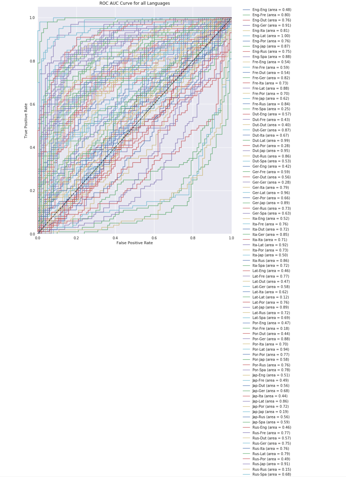
Because of the large number of lines in the plot, it is hard to discern what the different ROCs are, but we can see a good range of values such as those that are above the line, near the middle, and those on the other side. Let's plot the curves for only English to see a more cleaner plot.
plot_roc_auc(all_fpr, all_tpr, all_roc, "English", 10)

>>>
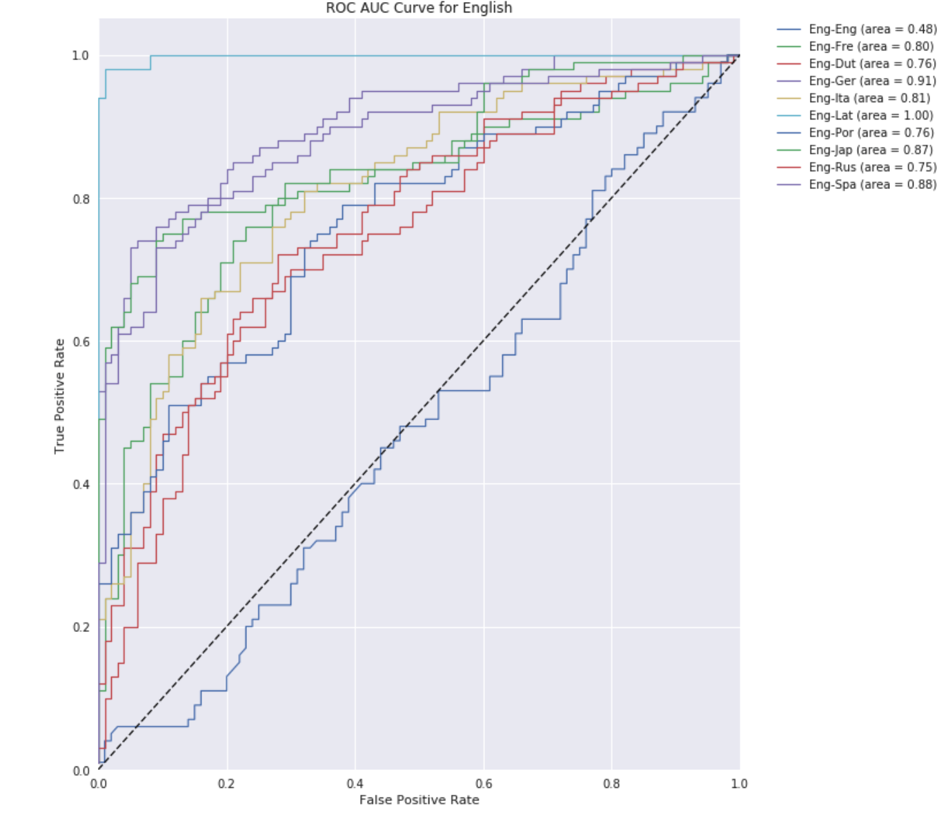
The plot shows that the only line that is around the line is the English-to-English curve, which makes sense because a well trained Neural Network will be unable to distinguish between two samples of the same language.
Results & Analysis
The ROC heatmap is a really interesting way to represent the interplay between languages. We can see clear trends in display. First, Latin consitently is the most easily differentiable of the languages with several high values and a max ROC of 0.96 in it's comparision to English. This shows us that the model did a great job of distinquishing between Latin and other languages.
Interestingly, Russian and Japanese are not very well distinguishable. This is very likely due to the Romanization process of the languages. The Romanized forms of these languages did not develop on their own but are artificially created. As a result, they are probably somewhat tame and constrained over a "true" language like Spanish or French.
Another aspect of the matrix is that we should expect the diagonal of the map to be around 0.50 as we cannot easily distinquish between two random samples of a single langugage. We see this trend as expected, minus a few outliers like Italian. This variability is caused by the random sampling used. Thoughout the project, we consistently found that there was a huge amount of variability in performance based on pure-luck. It seems as though one of the sample sets is very "Italian" while the other is not particulary remarkable. As a result, the models can more easily classifiy the samples. The ROC plots are self explanatory. For English, we see strong performance on all languages excluding the English-English comparison.
Code
To obtain the code please refer to this GitHub repository.
References:
- https://keras.io/getting-started/sequential-model-guide/
- https://github.com/fchollet/keras/blob/master/examples/lstm_text_generation.py
$\leftarrow$