Machine Learning
By: Adam Lieberman
Introduction:
This guide serves as a practicial guide to machine learning. It is meant to be concise, relaying some mathematical and theoretical ideals, as well as practical in nature. It is meant to get one up and running with machine learning and and cover the process of building a wide variety of machine learning algorithms.
Definition:
There are many different definitions of Machine Learning:
- Arthur Samuel (1956) - A field of computer science that gives computers the ability to learn without being explicitly programmed.
- Tom Mitchell (1998) - A computer program is said to learn from experience E with respect to some class of tasks T and performance measure P id its performance at tasks in T, as measured by P, improves with experience E.
There is not one correct definition for Machine Learning, but overall the idea of machine learning is that there are algorithms which can tell you intersting facets of your data without you specifically writing code by setting specific rules for the desired information. Ian Goodfellow provides a concise description: a machine learning algorithm is an algorithm that is able to learn form data.
Machine Learning in the AI Spectrum:
Machine Learning is a subset of artificial intelligence where we define artificial intelligence as the design of an intelligent agent that percieves its environment and makes decisions to maximize chances of achieving its goal. Here, machine learning is a subset of AI. The graphic below depicts the relationship between artificial intellignence, machine learning, and deep learning:
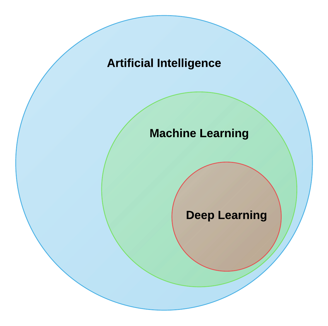
Machine Learning is a subset of Artificial Intelligence so all machine learning problems are artificial intelligence problems; however, not all artificial intelligence problems are machine learning problems. Artificial intelligence is not only concerned with algorithms learning from experience to data, but also having machines exhibit intelligence through rules and logic. This could, for instance, be finding an optimal path on a graph. Some alternate subfields of AI are as follows:
Machine Learning Principles
Structured vs Unstructured Data:
There are two types of data that can be used in machine learning models:
- Structured Data: information that can be ordered easily and processed by data mining tools. This is data that could be found in a database. Here, the information is organized and is easy to process. An example of structured data is as follows:
- Unstructured Data: data that is found in the "wild" which consists of free-form text, images, audio, and video. Here, the data has less structure, is not in a datbase, and does not adhere to a formal data model. An example of unstructured data is as follows:
| Ticker | Date | Price |
| AAPL | 09/01/2017 | 225.43 |
| AAPL | 09/02/2017 | 222.43 |
| AAPL | 09/03/2017 | 228.43 |
| today I wAs reading a book, it was good. |
| Tomorrow is going 2 be really nice. |
| I am playing basketball at 6:30 pm tomorrow. |
| It is a great day for a picnic. |
Feature Vectors:
In machine learning, an algorithm has to take in a feature vector to recieve an output. This is an $n$ dimensional vector of numerical features that represent some object. For example, say we have the following dataset of home prices and square feet:
| Price | Sq. Feet | Number of bedrooms |
| 220500.22 | 1245 | 3 |
| 125000.21 | 845 | 1 |
| 524589.55 | 3580 | 5 |
If we wish to be able to predict the price of a home given its square feet and number of bedrooms than we can have a two dimensional feature vector consist of the square feet and number of bedrooms. Our feature vectors for the above dataset would be: [1245, 3], [845,1], [3580,5]. We call the features that go into the model inputs and the result from inputting the features into the model the targets. The targets for the above example would be [220500.22],[12500.21],[524589.55]. Where each output corresponds to a target.
If we have categorical variables, we need to encode them into numerical quantities. Take for instance the following dataset:
| items |
| apple,banana |
| carrots |
| apple,carrots,rice,milk |
In order for our machine learning model to process this data, we have to convert it into a numerical quantity. To do so we could one-hot encode the variables. This means that we take a set of all items and create a vector with dimension that is the length of the set. For each item we have in the sample, we place a 1 in the corresponding index. The dataset above in one-hot encoded form would be as follows: [1,1,0,0,0],[0,0,1,0,0],[1,0,1,1,1] as our set of items is {apple, banana, carrots, rice, milk}. We see that index 0 corresponds to apple, index 1 to banana, and so on.
If we have a set of text documents, say tweets or emails, we might choose to count the number of times the words appear instead of one-hot encoding the words. This is an alterante type of feature we can use for text documents.
Function Mappings:
A function $f$ is a relation between a set of inputs and a set of outputs. In the housing price example above, each input had a specific output. We could create a function that maps the inputs to their outputs. This allows us to pass in a new unseen output and get a predicted output. We can visualize the process as follows:

An example of a function is $f(x) = x^2$. Here, we can let $9$ be an input and our output is $9^2 = 81$. Our machine learning algorithm could produce a function $f$ where we input an image and it maps the image to either cat or dog. The important thing to understand about function mappings is that a function $f$ takes an input and assigns it an output.
Machine Learning Tasks:
There are many different types of tasks that machine learning can solve:
- Classification: Classification deals with classifying an input into one of $k$ categories. We might, for instance, want to take a picture and decide whether it is a bird, cat, or dog. When we have more than two classes we have a "multiclass" classification problem. When we are looking at predicting two classes we have a "binary" classification problem. Mathematically speaking, the learning algorithm produces a function $f: \mathbb{R}^n \rightarrow \{1,2,...,k \}$. This notation means that we have an $n$ dimensional vector with values as real numbers that gets mapped to a discrete value in the set $\{1,2,...,k \}$ where $\{1,2,...,k\}$ are the classes of the classification problem. This function takes in a vector $x$ and outputs a value $y$ such that $f(x)=y$. An alternate variation of classification is where the function $f$ outputs a probability distribution over classes. For example, we would return a vector $v$ such as [.2,.7,.1] which means the probability that the input $x$ is class 1 is .2, the probability $x$ is class 2 is .7, and the probability $x$ is class 3 is .1. We can take the maximum value of this probability distribution over the classes to see that class 2 is the most probable classification for the input $x$. Classification produces discrete values. Discrete data can only take particular values. There may potentially be an infinite number of those values, but each is distinct and there's no grey area in between. Discrete data can be numeric like numbers of oranges, but it can also be categorical like red or blue or male or female.
- Classification with missing inputs: With regular classification above, each input vector $x$ has to have the same dimension. This means that if we have a sample $x_1$ = [5,13,4,5] then $x_2$ must have 4 values like $x_1$, making it a vector of dimension 4. If we do not have a gurantee that every measurement in the input vector will be provided then this makes classification more difficult. For a solution to this problem, we need the learning algorithm to define a single function mapping from the input vector to a categorical output. The learning algorithm learns a set of functions where each function corresponds to classifying the input $x$ with a different subset of its missing input values. If we have an $n$ dimensional feature vector than there will be $2^n$ different classification functions needed for each possible set of missing inputs.
- Regression: Regression tasks involve predicting a continuous value given an input $x$. Continuous data are not restricted to defined separate values, but can occupy any value over a continuous range. Between any two continuous data values there may be an infinite number of others. Continuous data are always essentially numeric. For instance, predicting the price of a stock is a regression problem since the value of the stock we predict could be any real number between 0 and infinity. Mathematically speaking, we take an input $x$ and pass it through a function $f:\mathbb{R}^n \rightarrow \mathbb{R}$ which means we take our $n$ dimensional input vector, pass it through the function $f$ and output a single real number.
- Transcription: Transcription involves the machine learning algorithm observing some unstructured data and transcribing it into a discrete textual form. For example, the algorithm might see an image of a license plate and transcribe it into text. Alternatively, the algorithm could be given a song and transcribe the audio into textual lyrics.
- Machine Translation: machine translations takes a sequence of symbols in one language and converts it into a sequence of symbols in another language. For example, converting a sentence from french to english. Google translate is an example of machine translation.
- Anomaly Detection: anomaly detection deals with the indentification of items, events, or observations which do not conform to an expected pattern or other items in a dataset. Here we search for unusual or atypical items in the dataset. For instance, looking for fradulent checks or identifying fraudlent credit card transactions are examples of anomaly detection.
- Synthesis and Sampling: With synthesis and sampling, the machine learning algorithm is asked to generate new examples that are similar to those in the training data. This is commonly used to generate data, such as healthcare data, which can be expensive to obtain or limited in size.
- Imputation of Missing Values: Here, the machine learning algorithm is given a sample $x$ and where some entries $x_i$ are missing and the algorithm must predict the missing entries.
- Clustering - Grouping samples of the data together.
Types of Machine Learning:
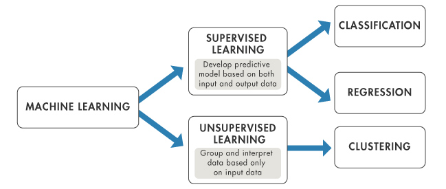
Machine learning algorithms can broadly be catagorized as either supervised or unsupervised learning problems. Unsupervised learning algorithms draw inferences from datasets consisting of input data without labeled responses (no targets). Here we want to discover an internal representation from the inputs only. With unsupervised learning there is no interest in prediction because there is not an associated response variable $y_i$ for each $x_i$. The goal is to discover interesting things about the data. It is typically used for the following tasks:
- Clustering - exploratory data analysis to find hidden patterns or grouping in data. The clusters are modeled using a measure of similarity which is defined upon metrics such as Euclidean or probabilistic distance.
- Dimensionality Reduction - Reducing the dimension of the input features in a manner that lets us still represent the true distribution of the dataset.
- Anomaly Detection - the identification of items, events or observations which do not conform to an expected pattern or other items in a dataset
Supervised learning algorithms observe a set of features $x_1,x_2,...,x_n$ as well as a label or a set of labels or target variables $y_1,y_2,...,y_n$ for each input. Supervised learning seeks to predict $y$ from $x$ by creating a function $f$ that takes an input $x$ and produces an output $y$ ($f(x) = y$). Supervised learning is typically used for the following tasks:
- Regression - predicting a value on a continuous domain.
- Classification - predicting what class a sample falls in.
</ol>
Supervised learning can be thought of as a teacher who shows a machine learning system what to do, while unspervised learning must make sense of the data without the instructor's help. The most common tasks for supervised learning are regression and clustering while the most common task for unsupervised learning is clustering. This can be summed up in the image below:
Math:
Mathematics is important in understanding how the algorithms work and why they work. In this section we cover some important principles from linear algebra, statistics, and information theory.
Programming:
The following is a list of machine learning libraries for their respective programming languages:
Python
- scikit-learn
- tebsorflow
- theano
- keras
- caffee
- pybrain
R
- caret
- RODBC
- Gmodels
- e1071
- glmnet
Java
- Weka
- MOA
- Deeplearning4j
- Mallet
- Elki
JavaScript
- brain.js
- Synaptic
- Mind
C++
- mlpack
- Tensorflow
- Dlib
- shogun
Julia
- MLBase.jl
- ScikitLearn.jl
- MachineLearning.jl
- Mocha.jl
Python is a great high-level language for rapid development of machine learning algorithms. It is used by many machine learning engineers, researchers, and developers in a wide variety of top companies and has many modules to assist in the machine learning process. All code in this guide will be written in python.
Performance Measure:
To evaluate the abilities of a machine learning algorithm, we must deisgn a quantitative measure of its performance. For classification tasks we often measure:
- Accuracy - the proportion of examples for which the model produces the correct output. This is the most common evaluation metric for classification problems
- Error Rate - the proportion of examples for which the model produces an incorrect output.
- Logarithmic Loss - A performance metric for evaluating the predictions of probabilities of membership to a given class. The scalar probability between 0 and 1 can be seen as a measure of confidence for a prediction by an algorithm.
- Area Under ROC Curve - A performance metric for binary classification problems. The AUC represents the model's ability to discriminate between positive and negative classes. An area of 1.0 represents a model that made all predictions perfectly. An area of 0.5 represents a model as good as random guesses.
- Confusion Matrix - A presentation of the accuracy of a model with two or more classes. The table presents predictions on the x-axis and accuracy outcomes on the y-axis. The cells of the table are the number of predictions made by a machine learning algorithm. Higher numbers on the diagonal indicate that more correct predictions were made than incorrect predictions.
For regression tasks there are three common metrics for evaluating predictions:
- Mean Absolute Error - The sum of the absolute differences between predictions and actual values. This gives an idea of how wrong the predictions were. Here, we get an idea of the magnitude of the error, but no idea of the direction (we cannot see if we were over or under predictig).
- Mean Squared Error - MSE measures the average of the squares of the errors or deviations, the difference between the estimator and what is estimated. For each pair of values we have $\Sigma_{i}^n (y_i - x_i)^2$. Here, we always get a positive number.
- Root Mean Squared Error - RMSE is the square root of the mean squared error.
- $R^2$ - a goodness of fit measure, how well the predictions align with the actual results as a value 0 (no fit) to 1 (perfect fit).
Train/Test Split:
We need to split our dataset into two groups: One group will be used to train the model and the second group will be used to measure the resulting model's error. We call this a train/test split. We pass the training data into the model so that the model learn's a subset of the data. We then evaluate the model on the test set so that we can see the performance of the model. This allows us to see performance in an unbiased way as we test our model on data that it has not seen.
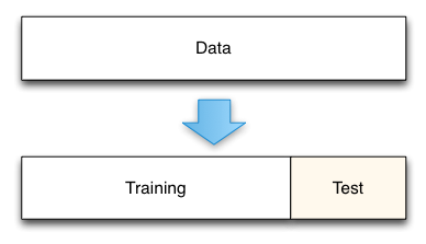
This technique is a gold standard for measuring the model's true prediction error. We typically use 80% of our data for the training set and 20% of our data for the testing set. If we have a non-time series dataset we typically choose random rows from our train set and test set. If our data is time-series we choose the first 80% of the rows of data for the train and the last 20% of the rows for testing.
Cross Validation:
Cross validation is a resampling technique that slits the data into $n$ folds. If we had 100 data points and we used 5-fold cross validation, we would create 5 folds with 20 data points each. The model building and error estimation process is repeated 5 times. Each of the 4 groups are combined to create 80 training data poitns. The 5th group of 20 data points is used to estimate the true prediction error. The process of cross validation (5-fold validation) is shown below:
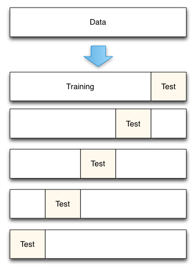
Cross validation is very similar to the holdout method. It is different in the sence that each data point is used both to train the model and to test the model, but never at the same time. When we have limited data, cross-validation is preferred to a train/test split as less data must be set aside in each fold than is needed in the pure holdout method. An important questions of cross-validation is what number of folds to use. If we have a smaller number of folds, then we have more bias in the error estimates, but the less variable they will be.
Overfitting/Underfitting:
The central challenge in machine learning is that our algorithm must perform well on new, previously unseen inputs. The ability to perform well on previously unobserved inputs is called generalization. The factors determining how well a machine learning algorithm will perform are its ability to:
- Make the training error small
- Make the gap between training and test error small
The above two factors correspond to the two central challenges in machine learning: underfitting and overfitting. Underfitting occurs when the model is not able to obtain a sufficiently low error value on the training set. Overfitting occurs when the gap between the training error and test error is too large.
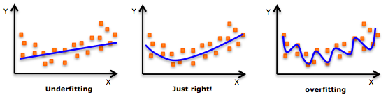
We can control wheter a model is more likely to overfit or underfit by altering its capacity. Models that overfit generally are too complex, having too many parameters relative to the number of observations. A model's capacity is its ability to fit a wide variety of functions. Models with low capacity may struggle to fit the training set. Models with high capacity can overfit by memorizing properties of the training set that do not serve them well on the test set. We can control the capacity of a learning algorithm by choosing its hypothesis space, the set of functions that the learning algorithm is allowed to select as being the solution. Machine learning algorithms will generally perform best when their capacity is appropriate for the true complexity of the task they need to perform and the amount of data they are provided with. Models with insufficient capacity are unable to solve complex tasks. Models with high capacity can solve complex tasks, but when their capacity is higher than needed to solve the present task, they may overfit.
Bias-Variance Tradeoff:
Understanding how different sources of error lead to bias and variance helps us improve the data fitting process, which results in more accurate models.
- Error due to Bias - The error due to bias is taken as the difference between the expected or average prediction of our model and the correct value which we are trying to predict. We only have one model, but can run our training and fitting multiple times. Due to randomness in the underlying datasets, the resulting model can have a range of predictions. Bias measures how far off in general these models' predictions are from the correct value.
- Error due to Variance - The error due to variance is how much the predictions for a given point vary between different realizations of the model.
We can depict the Bias-Variance Tradeoff as follows:
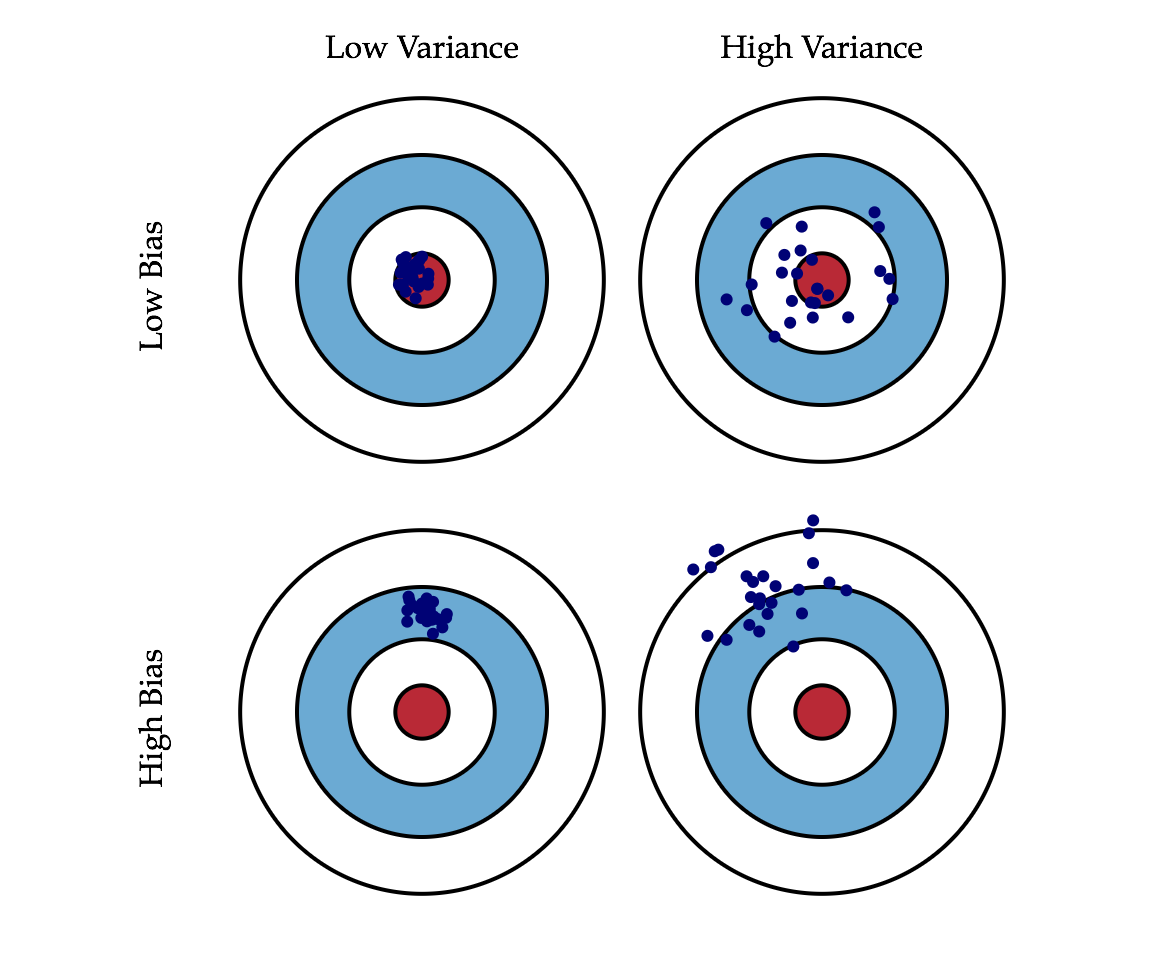
We can create a graphical visualization of bias and variance using a bulls-eye diagram. Imagine that the center of the target is a model that perfectly predicts the correct values. As we move away from the bulls-eye, our predictions get worse and worse. Imagine we can repeat our entire model building process to get a number of separate hits on the target. Each hit represents an individual realization of our model, given the chance variability in the training data we gather. Sometimes we will get a good distribution of training data so we predict very well and we are close to the bulls-eye, while sometimes our training data might be full of outliers or non-standard values resulting in poorer predictions. These different realizations result in a scatter of hits on the target.
At its root, dealing with bias and variance is really about dealing with over and underfitting. As a model becomes more complex, the bias is reduced and the variance increases. When we add more and more parameters to a model, the complexity increases and variance becomes our main concern.
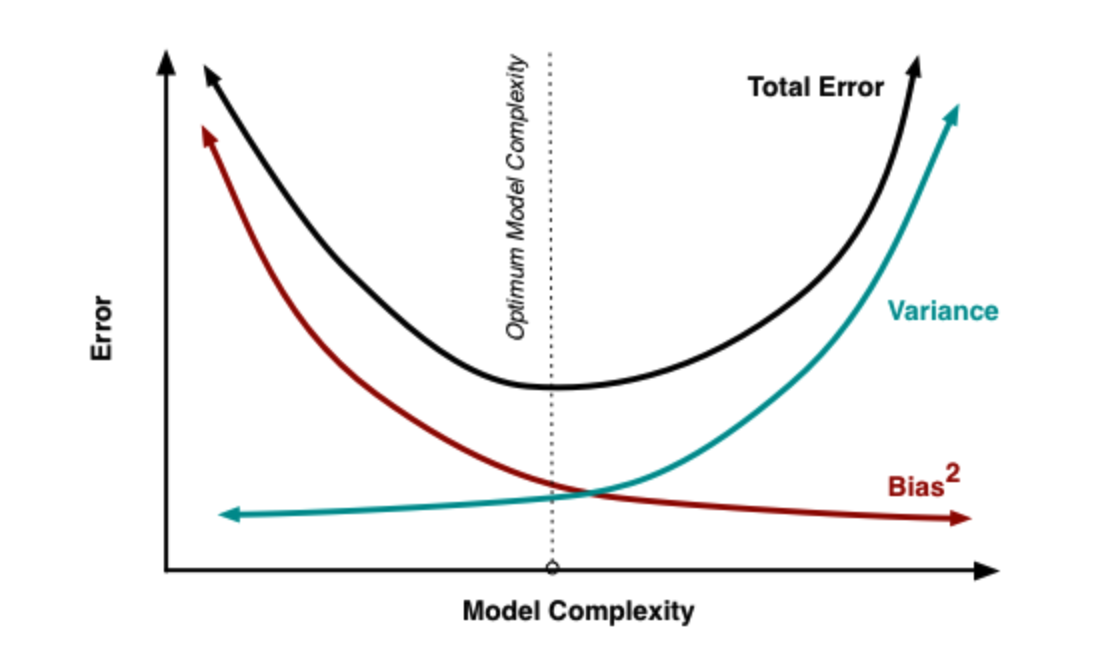
We want to hit the sweet spot where bias and variance intersect so that we do not overfit or underfit our model. In practice, there is not an analytical way to find this location. Instead we must use an accurate measure of prediction error and explore differing levels of model complexity and then choose the complexity level that minimizes the overall error.
Regularization:
Regularization is a way to correct overfitting by adding a pentalty on the different parameters of the model to reduce the freedom of the model. Hence, the model will be less likely to fir the noise of the training data and will improve generalization abilities of the model. There are a few popular regularization techniques:
- Lasso (L1 Regularization) - Adds an absolute value of magnitude of the coefficient as penalty term to the loss function. We add $\lambda \sum_{j=1}^p |\beta_j|$ to the loss function. Lasso shrinks the less important feature's coefficient to zero. This works well when we have a huge number of features and helps with feature selection, which L2 Regularization will not do.
- Ridge (L2 Regularization) - Adds squared magnitude of coefficient as penalty to the loss function. We add $\lambda \sum_{j=1}^p |\beta_{j}^2|$ as penalty to the loss function. L2 regularization generally gives better accuracy on unseen data comapred to L1 regularization. </ul>
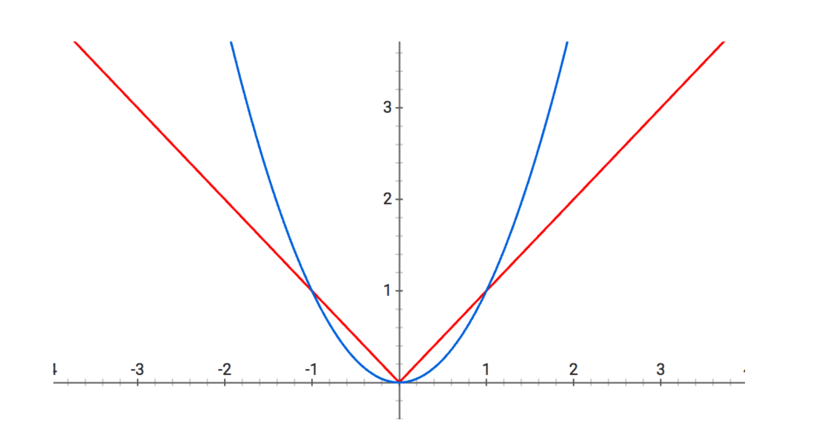
Above are plots of the absolute value and square functions. When minimizing a loss function with a regularization term, each of the entries in the parameter vector theta are “pulled” down towards zero. Think of each entry in theta lying on one the above curves and being subjected to “gravity” proportional to the regularization hyperparameter k. In the context of L1-regularization, the entries of theta are pulled towards zero proportionally to their absolute values — they lie on the red curve. In the context of L2-regularization, the entries are pulled towards zero proportionally to their squares — the blue curve.
At first, L2 seems more severe, but the caveat is that, approaching zero, a different picture emerges:
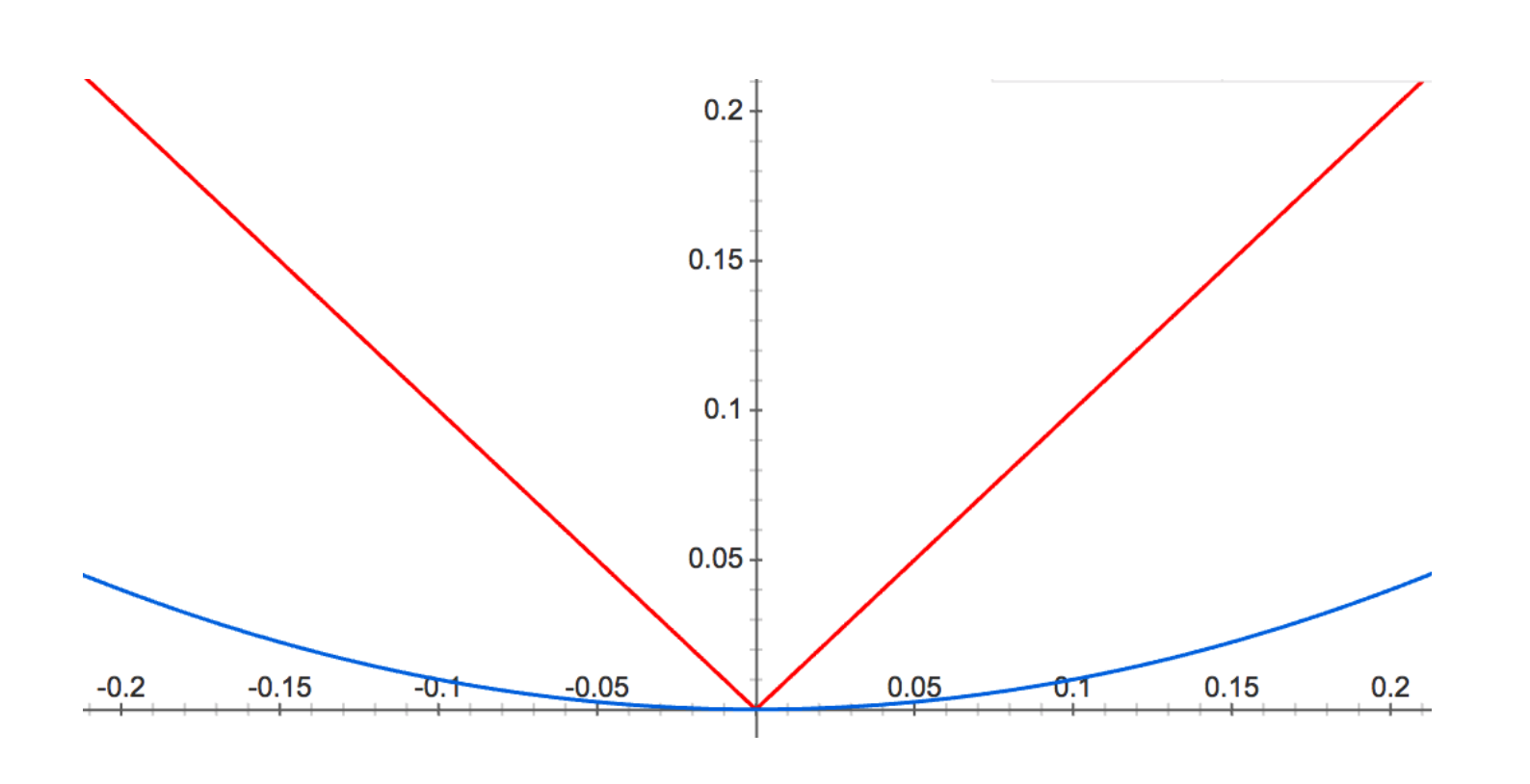
The result is that L2 regularization drives many of your parameters down, but will not necessarily eradicate them, since the penalty all but disappears near zero. Contrarily, L1 regularization forces non-essential entries of theta all the way to zero.
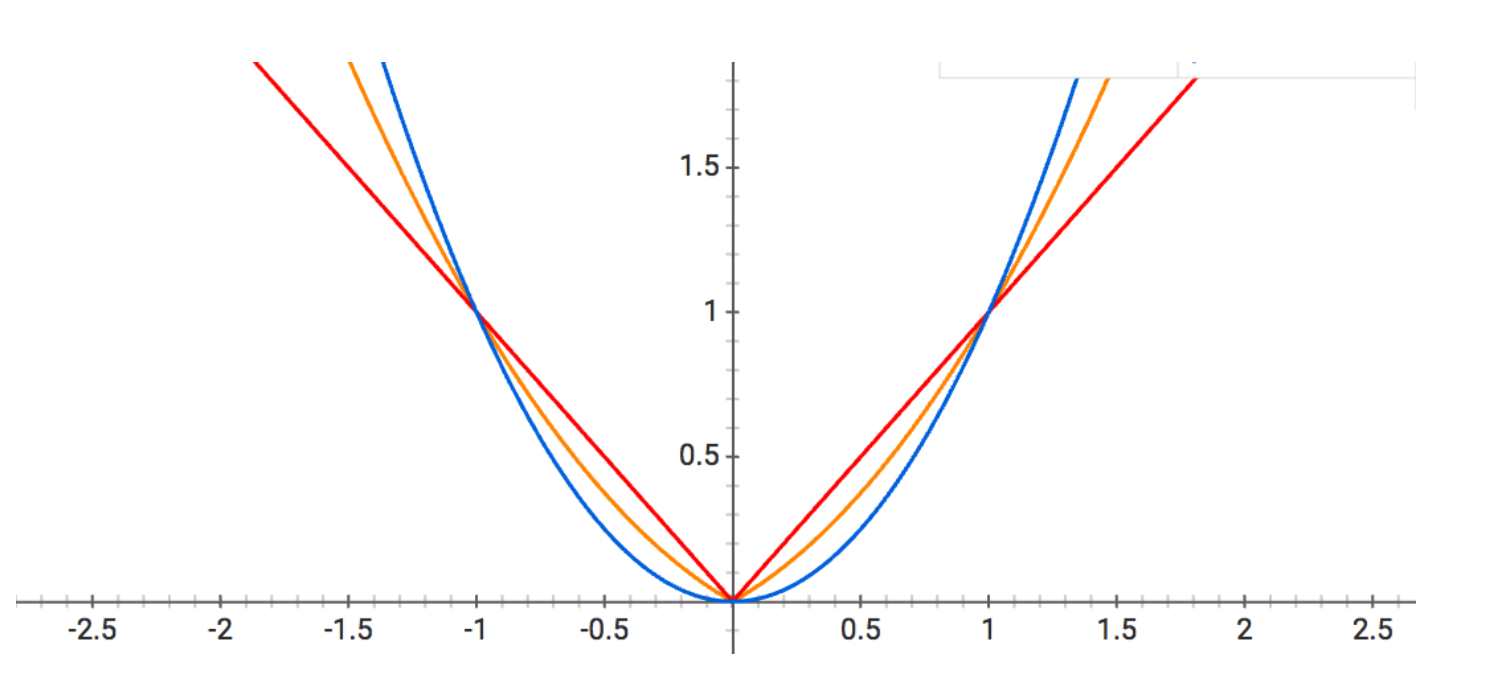
An alternate regularization technique is called ElasticNet, which is $\frac{L_1}{L_2}$. It is a compromise between Lasso and Ridge regression. It is depicted as the orange curve in the graph below:
The Curse of Dimensionality:
Machine learning problems become more difficult when the number of dimensions in the data is high. This phenomenon is known as the curse of dimensionality. This is of concern as the number of possible distinct configurations of a set of variables increases exponentially as the number of variables increases. An easy analogy is as follows: it is easy to catch a caterpillar moving in a tube (moving in 1 dimension). It is harder to catch a chicken running in a field (moving in 2 dimensions). It is even harder to catch two birds (moving in 3 dimensions). It is even harder to catch a ghost (moving in 3+ dimensions). Overall, the curse of dimensionality refers to how certain learning algorithms may perform poorly in high-dimensional data.
Feature Selection:
A key question in machine learning is which features we should use to create a predictive model. This is a difficult question and may require specific domain knowledge. Feature selection allows us to automatically select those features in our data that are most useful or most relevant for the problem we are working on. Feature selection is different from dimensionality reduction. Both methods seek to reduce the number of attributes in the dataset, but a dimensionality reduction method does so by creating new combinations of attributes, whereas a feature selection method includes and excludes attributes that are present in the data without changing them. We use feature selection methods to identify and remove unneeded, irrelevant, and redundant attributes from data that do not contribute to the accuracy of a predictive model or may in fact decrease the accuracy of the model. There are three general classes of feature selection algorithms:
- Filter Methods - Applying a statistical measure to score each feature. The features are ranked by score and either selected to be kept or removed from the dataset.
- Wrapper Methods - Consider the selection of features as a search problem, where different combinations are prepared, evaluated, and compared to other combinations.
- Embedded Methods - Learn which features best contribute to the accuracy of the model while the model is being created.
The No Free Lunch Theorem:
The no free lunch theorem for machine learning states that, averaged over all possible data-generating distributions, every classification algorithm has the same error rate when classifying previously unobserved points. In some sense, this means that no machine learning algorithm is universally better than any other. The most sophisticated algorithm we can concieve of has the same average perforamnce (over all possible tasks) as merely predicting that every point belongs to the same class. This only holds when we average over all possible data-generating distributions. If we take any two machine learning algorithms and average the performance across all possible problems, then neither algorithm will be better than one another. So, no one model works best for all possible situations. Models only work better for particular situations depending on how the data is distributed. Thus, we must design our machine learning algorithm to perform well on a specific task.
Parameters v.s. Hyperparameters:
- Model Parameter - A configuration variable that is internal to the model and whose value can be estimated by the data. These parameters are required by the model when making predictions, are often not manually set, and are often saved as part of the learned model. For example, the coefficients in a linear regression or logistic regression model.
- Model Hyperparameter - A configuration that is external to the model and whose value cannot be estimated from the data. These are often specified by the engineer and are often tuned for a given predictive modeling problem. For example, the K in K-Nearest Neighbors or the learning rate for training a neural network. </ul>
A general rule of thumb is that "if you have to specify a model parameter manually then it is probably a model hyperparameter." In summary, model parameters are estimated from data automatically and model hyperparameters are set manually and are used in processes to help estimate model parameters.
Occam's Razor:
Many early scholars invoke a principle of parsimony that is now widely known as Occam's Razor. This principle states that among competing hypotheses that explain known observations equally well, we should choose the "simplest" one. If we have two models that have the same performance, we should choose the simpler model.
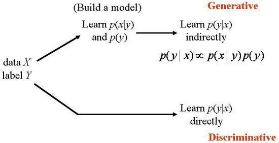
Generative v.s. Discriminative Algorithms:
- Generative Algorithm - Models how the data was generated in order to categorize a signal. It asks the question "Based on my generation assumptions, which category is most likely to generate this signal?" Here, we find the likelihood that the input is of one class and choose the class that has the highest probability. For example: Gaussian, Naive Bayes
- Discriminative Algorithm - Models that do not care how the data was generated, they simply categorize a given signal. Here we just create a decision boundary between classes and whatever area the input falls into is the class assigned to it. For example: Logistic Regression, SVMs, KNN </ul>
Machine Learning Pipeline:
The general machine learning pipeline is as follows:
- Get access to data
- Clean/Preprocess Data
- Analyze data
- Generate Features
- Feature Selection
- Create Train/Test split or use cross validation
- Choose Model
- Train model with
- Evaluate model with test data
- Tune model
- Repeat steps 7-10
Feature Selection
Algorithms for for feature selectionUnivariate Statistical Test using Chi-Squared for Classification:
import pandas
import numpy
from sklearn.feature_selection import SelectKBest
from sklearn.feature_selection import chi2
# load data
url = "https://archive.ics.uci.edu/ml/machine-learning-databases/pima-indians-diabetes/pima-indians-diabetes.data"
names = ['preg', 'plas', 'pres', 'skin', 'test', 'mass', 'pedi', 'age', 'class']
dataframe = pandas.read_csv(url, names=names)
array = dataframe.values
X = array[:,0:8]
Y = array[:,8]

# feature extraction
test = SelectKBest(score_func=chi2, k=4)
fit = test.fit(X, Y)

# summarize scores
numpy.set_printoptions(precision=3)
print("Feature Scores: ",fit.scores_)
best_features = np.argsort(np.array(fit.scores_))[::-1][:]
ls_best_features = [names[i] for i in best_features]
print('Features Best to worst: ',ls_best_features)

features = fit.transform(X)
# summarize selected features
new_data = features
Recursive Feature Elimination:
Recursively remove attributes and build a model on the attributes that remain:
from pandas import read_csv
from sklearn.feature_selection import RFE
from sklearn.linear_model import LogisticRegression
# load data
url = "https://archive.ics.uci.edu/ml/machine-learning-databases/pima-indians-diabetes/pima-indians-diabetes.data"
names = ['preg', 'plas', 'pres', 'skin', 'test', 'mass', 'pedi', 'age', 'class']
dataframe = read_csv(url, names=names)
array = dataframe.values
X = array[:,0:8]
Y = array[:,8]

# feature extraction
model = LogisticRegression()
rfe = RFE(model, 3)
fit = rfe.fit(X, Y)
selected_features = np.array(names)[fit.support_]
print("Number of features: ", fit.n_features_)
print("Selected Features: ", selected_features)
print("Feature Ranking: ", fit.ranking_) #Choice is 1 if we should select the feature
Classification Algorithms
Building models for supervised classificationSupport Vector Machine (SVM):
#Imports
import numpy as np
import pandas as pd
from sklearn import svm
from sklearn.datasets.samples_generator import make_blobs, make_classification
from sklearn.model_selection import train_test_split
from sklearn.metrics import accuracy_score
#Load Data
X, y = make_blobs(n_samples=10000, centers=2, n_features=2,random_state=0)

#Create random train/test split
X_train, X_test, Y_train, Y_test = train_test_split(X, y, test_size=0.25, random_state=42)
svm_model = svm.SVC()
svm_model.fit(X_train,Y_train)
preds = svm_model.predict(X_test)
acc = accuracy_score(Y_test,preds)
print('accuracy: ',acc*100, '%')
K-Nearest Neighbors:
from sklearn.neighbors import KNeighborsClassifier
X, y = make_classification(n_samples=1000, n_classes=4, n_features=4,n_informative=3, n_redundant=0,random_state=0, shuffle=False)
X_train, X_test, Y_train, Y_test = train_test_split(X, y, test_size=0.25, random_state=42)
knn = KNeighborsClassifier(n_neighbors=3)
knn.fit(X_train,Y_train)
preds = knn.predict(X_test)
acc = accuracy_score(Y_test,preds)
print('accuracy: ',acc*100, '%')
Gaussian Discriminative Analysis (GDA):
from sklearn.gaussian_process import GaussianProcessClassifier
X, y = make_classification(n_samples=1000, n_classes=3, n_features=4,n_informative=3, n_redundant=0,random_state=0, shuffle=False)
X_train, X_test, Y_train, Y_test = train_test_split(X, y, test_size=0.25, random_state=42)
g = GaussianProcessClassifier()
g.fit(X_train,Y_train)
preds = g.predict(X_test)
acc = accuracy_score(Y_test,preds)
print('accuracy: ',acc*100, '%')
Naive Bayes:
from sklearn.naive_bayes import GaussianNB
X, y = make_classification(n_samples=1000, n_classes=3, n_features=40,n_informative=3, n_redundant=0,random_state=0, shuffle=False)
X_train, X_test, Y_train, Y_test = train_test_split(X, y, test_size=0.25, random_state=42)
nb = GaussianNB()
nb.fit(X_train,Y_train)
preds = nb.predict(X_test)
acc = accuracy_score(Y_test,preds)
print('accuracy: ',acc*100, '%')
Decision Tree:
from sklearn.tree import DecisionTreeClassifier
X, y = make_classification(n_samples=25000, n_classes=3, n_features=40,n_informative=3, n_redundant=0,random_state=0, shuffle=False)
X_train, X_test, Y_train, Y_test = train_test_split(X, y, test_size=0.25, random_state=42)
dt = DecisionTreeClassifier(criterion='entropy')
dt.fit(X_train,Y_train)
preds = nb.predict(X_test)
acc = accuracy_score(Y_test,preds)
print('accuracy: ',acc*100, '%')
Random Forest:
from sklearn.ensemble import RandomForestClassifier
X, y = make_classification(n_samples=10000, n_classes=3, n_features=20,n_informative=3, n_redundant=0,random_state=0, shuffle=False)
X_train, X_test, Y_train, Y_test = train_test_split(X, y, test_size=0.25, random_state=42)
rf = RandomForestClassifier(n_estimators=100, criterion='gini',max_depth=2, random_state=0)
rf.fit(X_train, Y_train)
preds = rf.predict(X_test)
acc = accuracy_score(Y_test,preds)
print('accuracy: ',acc*100, '%')
Logistic Regression:
from sklearn.linear_model import LogisticRegression
X, y = make_classification(n_samples=1000, n_classes=2, n_features=2,n_informative=2, n_redundant=0,random_state=0, shuffle=False)
X_train, X_test, Y_train, Y_test = train_test_split(X, y, test_size=0.25, random_state=42)
lr = LogisticRegression()
lr.fit(X_train,Y_train)
preds = lr.predict(X_test)
acc = accuracy_score(Y_test,preds)
print('accuracy: ',acc*100, '%')
Regression Algorithms
Building models for supervised regressionLinear Regression:
from sklearn.linear_model import LinearRegression
from sklearn.datasets import make_regression
from sklearn.metrics import mean_squared_error
X,y = make_regression(n_samples=20000,random_state=0)
X_train, X_test, Y_train, Y_test = train_test_split(X, y, test_size=0.25, random_state=42)
lr = LinearRegression()
lr.fit(X_train,Y_train)
preds = lr.predict(X_test)
mse = mean_squared_error(Y_test,preds)
print('mse: ',mse)
Polynomial Regression:
import numpy as np

from sklearn.pipeline import Pipeline
from sklearn.preprocessing import PolynomialFeatures
from sklearn.linear_model import LinearRegression
from sklearn import cross_validation
X,y = make_regression(n_samples=200, n_features=3, n_informative=3,random_state=0)
X_train, X_test, Y_train, Y_test = train_test_split(X, y, test_size=0.25, random_state=42)

polynomial_features = PolynomialFeatures(degree=3,include_bias=False)
linear_regression = LinearRegression()
pipeline = Pipeline([("polynomial_features", polynomial_features),("linear_regression", linear_regression)])
pipeline.fit(X_train, Y_train)

# Evaluate the models using cross validation
scores = cross_validation.cross_val_score(pipeline,X_train, Y_train, scoring="mean_squared_error", cv=2)

print("Cross Validation Scores: ", scores)
scores_test = pipeline.predict(X_test)
preds = pipeline.predict(X_test)
mse = mean_squared_error(Y_test,preds)
print("Test set MSE: ", mse)
Decision Trees:
from sklearn.tree import DecisionTreeRegressor
from sklearn.model_selection import cross_val_score
from sklearn.datasets import load_boston
boston = load_boston()
X = boston.data
y = boston.target
X_train, X_test, Y_train, Y_test = train_test_split(X, y, test_size=0.2, random_state=42)

dtr = DecisionTreeRegressor(criterion='mse',splitter='best',max_depth=None)
dtr.fit(X_train,Y_train)
preds = dtr.predict(X_test)
mse = mean_squared_error(Y_test,preds)
print('mse: ',mse)

cv_scores = cross_val_score(dtr, boston.data, boston.target, cv=10)
print("cross validation scores: ", cv_scores)
Random Forests:
from sklearn.ensemble import RandomForestRegressor
from sklearn.datasets import make_regression
from sklearn.metrics import mean_squared_error
X,y = make_regression(n_samples=20000, n_features=2, n_informative=3,random_state=0)
X_train, X_test, Y_train, Y_test = train_test_split(X, y, test_size=0.2, random_state=42)

rfr = RandomForestRegressor(n_estimators = 100,max_depth=50, random_state=0)
rfr.fit(X_train,Y_train)
preds = rfr.predict(X_test)
mse = mean_squared_error(Y_test,preds)
print('mse: ',mse)
Support Vector Regression:
from sklearn.svm import SVR
from sklearn.datasets import load_boston
from sklearn.metrics import mean_squared_error
X,y = make_regression(n_samples=20000, n_features=2, n_informative=2,random_state=0)
X_train, X_test, Y_train, Y_test = train_test_split(X, y, test_size=0.2, random_state=42)

svr = SVR(kernel='rbf', C=1e3, gamma=0.1)
svr.fit(X_train,Y_train)
preds = svr.predict(X_test)
mse = mean_squared_error(Y_test,preds)
print('mse: ',mse)
Regularization Algorithms
Building models for supervised regressionLasso Regularization with Linear Regression:
from sklearn import datasets, linear_model
from sklearn.model_selection import cross_val_score
from sklearn.datasets import load_diabetes
diabetes = datasets.load_diabetes()
X = diabetes.data[:150]
y = diabetes.target[:150]
X_train, X_test, Y_train, Y_test = train_test_split(X, y, test_size=0.2, random_state=42)
lasso = linear_model.Lasso()
lasso.fit(X_train,Y_train)
print(cross_val_score(lasso, X_test, Y_test))
Ridge Regression with Linear Regression:
from sklearn import datasets, linear_model
from sklearn.model_selection import cross_val_score
from sklearn.datasets import load_diabetes
diabetes = datasets.load_diabetes()
X = diabetes.data[:150]
y = diabetes.target[:150]
X_train, X_test, Y_train, Y_test = train_test_split(X, y, test_size=0.2, random_state=42)
lasso = linear_model.Ridge()
lasso.fit(X_train,Y_train)
print(cross_val_score(lasso, X_test, Y_test))
Clustering Algorithms
Building models for unsupervised clusteringK-Means:
from sklearn.datasets import load_breast_cancer
from sklearn.cluster import KMeans
from matplotlib import pyplot as plt
import numpy as np
X = load_breast_cancer()
data = X.data
k = 2
kmeans = KMeans(n_clusters=k)
kmeans.fit(data)
labels = kmeans.labels_
centroids = kmeans.cluster_centers_

for i in range(k):
    # select only data observations with cluster label == i
    ds = data[np.where(labels==i)]
    # plot the data observations
    plt.plot(ds[:,0],ds[:,1],'o')
    # plot the centroids
    lines = pyplot.plot(centroids[i,0],centroids[i,1],'kx')
    # make the centroid x's bigger
    plt.setp(lines,ms=15.0)
    plt.setp(lines,mew=2.0)
    plt.title("KMeans predictions (k=2)")
plt.show()

Affinity Propogation:
from sklearn.datasets import make_blobs
from sklearn.cluster import AffinityPropagation
from matplotlib import pyplot as plt
from sklearn import metrics

import numpy as np
from itertools import cycle
centers = [[1, 1], [-1, -1], [1, -1]]
X, labels_true = make_blobs(n_samples=300, centers=centers, cluster_std=0.5, random_state=0)

af = AffinityPropagation(preference=-50).fit(X)
cluster_centers_indices = af.cluster_centers_indices_
labels = af.labels_


n_clusters_ = len(cluster_centers_indices)

print("Clustering Metrics:")
print('Estimated number of clusters: %d' % n_clusters_)
print("Homogeneity: %0.3f" % metrics.homogeneity_score(labels_true, labels))
print("Completeness: %0.3f" % metrics.completeness_score(labels_true, labels))
print("V-measure: %0.3f" % metrics.v_measure_score(labels_true, labels))
print("Adjusted Rand Index: %0.3f"
      % metrics.adjusted_rand_score(labels_true, labels))
print("Adjusted Mutual Information: %0.3f"
      % metrics.adjusted_mutual_info_score(labels_true, labels))
print("Silhouette Coefficient: %0.3f"
      % metrics.silhouette_score(X, labels, metric='sqeuclidean'))

plt.figure(1)
plt.clf()

colors = cycle('bgrcmykbgrcmykbgrcmykbgrcmyk')
for k, col in zip(range(n_clusters_), colors):
    class_members = labels == k
    cluster_center = X[cluster_centers_indices[k]]
    plt.plot(X[class_members, 0], X[class_members, 1], col + '.')
    plt.plot(cluster_center[0], cluster_center[1], 'o', markerfacecolor=col,
             markeredgecolor='k', markersize=14)
    for x in X[class_members]:
        plt.plot([cluster_center[0], x[0]], [cluster_center[1], x[1]], col)

plt.title('Estimated number of clusters: %d' % n_clusters_)
plt.show()

Dimensionality Reduction Algorithms
Building models for unsupervised dimensionality reductionPrincipal Component Analysis (PCA):
import numpy as np
from sklearn.decomposition import PCA
import numpy as np
from sklearn.decomposition import PCA

# gaussian random variable, 10-dimension, identity cov mat
X = np.random.randn(100000, 10)
print("Original Dimension: ", X.shape)
pca = PCA(n_components=5)
X_transformed = pca.fit_transform(X)

print("Dimensionality Reduction Dimension: ",X_transformed.shape)
from sklearn.datasets import fetch_lfw_people
lfw_people = fetch_lfw_people(min_faces_per_person=70, resize=0.4)

n_samples, h, w = lfw_people.images.shape
X = lfw_people.data
y = lfw_people.target
X_train, X_test, y_train, y_test = train_test_split(X, y, test_size=0.25, random_state=42)

n_components = 200
pca = PCA(n_components=n_components, svd_solver='randomized',whiten=True)
pca.fit(X_train)

eigenfaces = pca.components_.reshape((n_components, h, w))
plt.imshow(eigenfaces[5])
plt.show()

plt.imshow(X_test[5].reshape(h,w))
plt.show()

