Background
I was recently given the following toy dataset:
annotated hamlet published in
shakespeare's hamlet
harry potter and the chamber of secrets
harry potter and the sorcerer's stone first edition
romeo and juliet
a first edition romeo and juliet
shakespeare's romeo and juliet
to kill a mockingbird
1984
orwell's 1984
king lear
an old copy of 1984
Above there are full book titles and fragments of book titles and the goal is to cluster the books that are similar e.g. cluster Harry Potter books from 1984 books from Romeo and Juilet books.
Libraries:
The following contains all libraries found in the code segments below:
import requests
import re
from bs4 import BeautifulSoup
import random
import numpy as np
import pandas as pd

import nltk
from nltk.corpus import stopwords

from sklearn.feature_extraction.text import CountVectorizer
from sklearn.feature_extraction.text import TfidfTransformer
from sklearn.cluster import KMeans
from sklearn.decomposition import PCA
Data:
Initially I looked for a full dataset for this problem, but there did not seem to be a set of book titles with altered book titles dataset. So, I decided to create my own small dataset. To do so I first scraped the 100 recommended book titles to read from Amazon using the requests package and BeautifulSoup. The code is as follows:
link = "https://www.amazon.com/b?ie=UTF8&node=8192263011"
html = requests.get(link).text
bs = BeautifulSoup(html,"html.parser")
books = []
for link in bs.find_all("span",{"class":"a-size-small"}):
    books.append(link.text)
Now that we have 100 book titles, we can randomly choose a starting point for each book title and a random length for each book title and create 5 modified titles for each book title. Additionally, there are 14 books in Amazon's list which have less than or equal to 2 words, so we filter these out. We create our 5 modified book titles for each book as follows and keep lables according to which modified books belong in the same cluster as the original book title so that we can evaluate our clustering later on. We do so as follows:
book_labels = []
modified_labels = []
modified_books = []
lbl = 0
for i in books:
    token_book = i.split()
    word_len = len(token_book)
    book_labels.append(lbl)
    #Filter out books of length <= 2
    if len(token_book) > 2:
        for j in range(5):
            random_start = random.randint(0,word_len-1)
            random_word_len = random.randint(2,word_len-1)
            if (random_start+random_word_len) > len(token_book[random_start:]):
                b_start = token_book[random_start:]
                b_end = token_book[0:random_word_len - len(b_start)]
                b = b_start + b_end
            else:
                b = token_book[random_start:(random_start+random_word_len)]
            modified_labels.append(lbl)
            modified_books.append(' '.join(b))
    lbl = lbl+1
After doing so we have 435 modified books and 100 regular book titles. We can now add the two lists together and create one list of all titles. We can additionally do the same for the cluster labels. We do so as follows:
all_titles = books+modified_books
all_labels = book_labels+modified_labels
We now have 535 book titles. We note that this is a small dataset.
Preprocessing:
We now need to preprocess our data. We need our data to have a uniform format and be machine readable so we keep only letters and numbers (0-9), lowercase all letters, tokenize the words, and remove stop words (words that serve no importance). We will write a function called clean_data which takes in a book title and returns the cleaned book title. The function is as follows:
def clean_data(raw_text):
    letters = re.sub("[^a-zA-Z0-9]", " ",raw_text)                #Keeps only letters and numbers
    lower_case = letters.lower()                                  #Keeps all words lowercase
    tok = lower_case.split()                                      #Tokenizes
    stop_words = set(stopwords.words("english"))                  #Create set of stopwords
    wrds = [w for w in tok if w not in stop_words]                #Removes stopwords
    return(" ".join(wrds))
We can now create a pandas dataframe of our book titles and use an apply and lambda to clean each book title and then extract a numpy array of our cleaned book titles. We do so as follows:
#Create pandas dataframe of all book titles
df_data = pd.DataFrame(all_titles,columns=['Book_Title'])

#Apply cleaning function on dataframe
df_data["cleaned_data"] = df_data["Book_Title"].apply(lambda i: clean_data(i))

#Numpy array of cleaned data
cleaned_data = df_data["cleaned_data"].values
We now have our preprocessed book titles:
Feature Generation:
Now that we have our cleaned book titles, we need to generate features for each book title. A popular feature is term frequency-inverse document frequency (tf-idf). Tfidf is a numerical statistic that is intended to reflect how important a word is to a document in a collection or corpus. We can caluclate the term frequency of a term, $t$, as $$TF(t) = \frac{\text{the number of times}\; t \; \text{appears in a document}}{\text{total number of terms in the document}}$$
We can calculate the inverse document frequency as: $$IDF(t) = \text{log}\left(\frac{\text{Total number of documents}}{\text{Number of documents with the term}\; t \; \text{in it}}\right)$$
For example, say we have a document that has 100 words and the word "dog" appears 3 times. The term frequenct for dog, $TF(\text{dog}) = \frac{3}{100} = 0.03$. Now, say we have 10,000,000 documents and the word "dog" appears in 1,000 of these. Then the inverse docment frequency $IDF(\text{dog}) = \text{log}\left(\frac{10,000,000}{1,000}\right) = 4$. Now, the tfidf score can be calculated as $0.03*4 = 0.12$.
There are some pros and cons of using tf-idf which we highlight below:
- Pros:
- Easy to compute
- Have a basic metric to extract the most descriptive terms of a document
- Can easily compute the similarity between 2 documents
- Great for nearly identical documents
- Cons:
- Does not capture position in text
- Does not capture semantics
- Documents that do not have a majority of similar words can perform poorly
Since our documents contain similar words, we will carry on forward using tf-idf feature vectors. We can use sklearn to create a count vectorizer and fit our data to it. We can then create a tf-idf transformer and fit the counts to it to obtain our tf-idf features. We do so as follows:
vectorizer = CountVectorizer(analyzer="word",tokenizer=None,preprocessor=None,stop_words=None)
vec_features = vectorizer.fit_transform(cleaned_data)  #The counts
X_counts = vec_features.toarray()
transformer = TfidfTransformer(smooth_idf=False)   #Create transformer
X_tfidf = transformer.fit_transform(X_counts)     #Fit transformer on the counts
X_tfidf = X_tfidf.toarray()
We now have our tf-idf feature vectors for all of our book titles.
K-Means Clustering:
Now that we have our features we need to cluster them. KMeans clustering is an unsupervised learning algorithm that partitions $n$ samples into $k$ clusters. We randomly create $k$ centroids, one for each cluster. These centroids are the mean locations of our clusters. We then take each point in the data set and associate it to the nearest centroid. Once all points are assigned we can recalculate the positions of the $k$ centroids. We then re assign all the points and repeat the process of updating the centroid position until no points move from the previous clustering assignment to the next. This produces a separation of the objects into groups from which the metric to be minimized can be calculated.
We can visually see this process as follows:
We see that at each iteration the stars, representing the centroid for each cluster, are adjusted and new data is shifted into the clusters.
Using sklearn we can easily instantiate a KMeans object and then fit our data to it as follows:
k = 100     #1 cluster for each book
km = KMeans(n_clusters=k, init='k-means++', max_iter=100)
km.fit(X_tfidf)
We can now create a cluster map so that we can print out the book titles assigned to each cluster. To do so we create a pandas dataframe and then let one column have the book titles and the other column have the cluster numbers, which we can obtain using the .labels_ function from sklearn. We do so as follows:
cluster_map = pd.DataFrame()
cluster_map['data_index'] = list(df_data["Book_Title"].values)
cluster_map['cluster'] = km.labels_
We can now print out the first 4 rows in our dataframe:
print(cluster_map.head(4))

>>>
                              data_index  cluster
0                 1984 (Signet Classics)       34
1                A Brief History of Time        2
2  A Heartbreaking Work of Staggering...       74
3   A Long Way Gone: Memoirs of a Boy...       66
We see each title has a corresponding cluster.
We can now print the following book titles per cluster using the following code:
for i in range(100):
    print("Cluster", i,": \n",cluster_map[cluster_map.cluster == i],"\n")
Let us look at cluster 64. This cluster should contain all book titles similar to "The Golden Compass: His Dark Materials". Below are the book titles in this cluster:
Cluster 64 :
                                  data_index  cluster
65   The Golden Compass: His Dark Materials       64
375                Golden Compass: His Dark       64
376                      Dark Materials The       64
378                      Dark Materials The       64
379                      His Dark Materials       64
We see that this cluster contains books that are similar to the book title.
Let us look at cluster 5. This cluster should contain all book titles similar to "Harry Potter and the Sorcerer's Stone". The results are as follows:
Cluster 5 :
                                 data_index  cluster
28   Harry Potter and the Sorcerer's Stone        5
210                 Sorcerer's Stone Harry        5
211        Potter and the Sorcerer's Stone        5
212                            Stone Harry        5
213        Harry Potter and the Sorcerer's        5
214             the Sorcerer's Stone Harry        5
Performance - Purity:
By examining the results by eye, we see that we did a pretty good job. The items in the clusters make sense as we see a lot of similar book titles clustered together. However, let us use a clustering performance metric called purity to quantitatively evaluate our clustering. To compute purity, each cluster is assigned to the class which is most frequent in the cluster, and then the accuracy of this assignment is measured by counting the number of correctly assigned documents and dividing by $N$. Mathematically speaking, $$\text{purity}\left(A,B\right) = \frac{1}{N}\sum_k \max_j |w_k \cap c_j|$$ where $A = {w_1,w_2,...,w_k}$ is the set of clusters and $B = {c_1,c_2,...,c_j}$ is the set of classes.
Let us look at the following example to better understand purity:
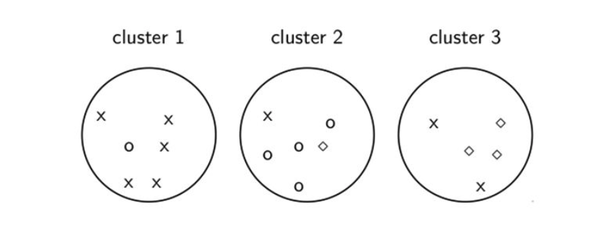
In the above figure the x belongs to cluster 1, the circle belongs to cluster 2, and the diamond belongs to cluster 3. We see that we had 5 x's correctly classified in cluster 1 so $5 = max_j | w_1 \cap c_j|$. In cluster 2 we had 4 circles correctly classified so $4 = max_j |w_2 \cap c_j|$. In cluster 3 we had 3 diamond's correctly classified so $3 = \max_j | w_3 \cap c_j|$. We can count all of the x's, circles, and diamonds and we see that $N = 17$. Thus, purity = $\frac{1}{17} \left(5+4+3 \right) \approx 0.71.$
Let us now write the following python function to compute purity:
def purity_score(clusters, classes):

    A = np.c_[(clusters,classes)]

    n_accurate = 0.

    for j in np.unique(A[:,0]):
        z = A[A[:,0] == j, 1]
        x = np.argmax(np.bincount(z))
        n_accurate += len(z[z == x])

    return n_accurate / A.shape[0]
We can now pass in the clusters from the KMeans algorithm and our labels (classes that we previously stored) and print our purity:
print("Purity: ",purity_score(km.labels_,all_labels))

>>>
Purity:  0.9102803738317757
We see that our purity was ~0.91. If our clustering algorithm did a perfect job our purity would be 1.0. Our purity value is very high and is a good indicator that our clustering did a good job.
Conclusion:
Looking across all 100 book title clusters we see that KMeans with tf-idf features worked well. This highlights the case that if we have to cluster short text documents where there are some nearly identical words in each document then using tf-idf with KMeans is not a problem. If for instance, we had 140 character tweets, tf-idf and KMeans might not give us great clustering as there may not be many words in common across tweets clustered based on user.
Code:
All code found in this tutorial can be found here.